

The Low Power of Cointegration Tests
One of the perennial difficulties in developing statistical arbitrage strategies is the lack of reliable methods of estimating a stationary portfolio comprising two or more securities. In a prior post (below) I discussed at some length one of the primary reasons for this, i.e. the lower power of cointegration tests. In this post I want to explore the issue in more depth, looking at the standard Johansen test Procedure to estimate cointegrating vectors.

Johansen Test for Cointegration
Start with some weekly data for an ETF triplet analyzed in Ernie Chan’s book:
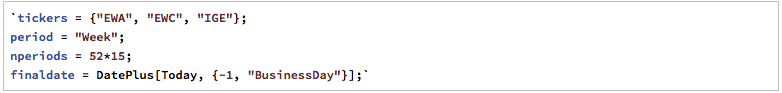
After downloading the weekly close prices for the three ETFs we divide the data into 14 years of in-sample data and 1 year out of sample: 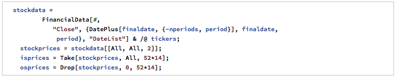
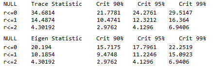
We next apply the Johansen test, using code kindly provided by Amanda Gerrish:
![]()
We find evidence of up to three cointegrating vectors at the 95% confidence level:
Let’s take a look at the vector coefficients (laid out in rows, in Amanda’s function):
![]()
In-Sample vs. Out-of-Sample testing
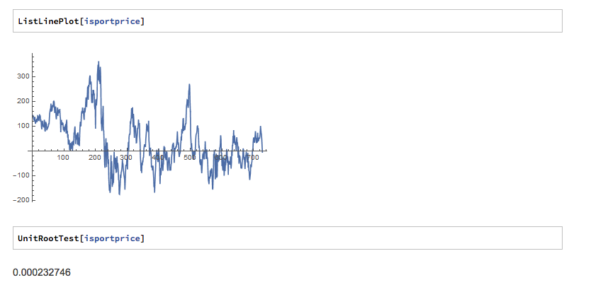
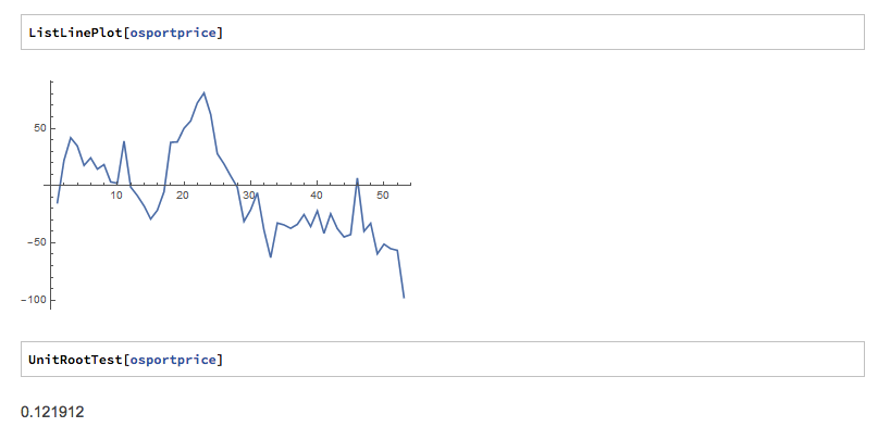
We now calculate the in-sample and out-of-sample portfolio values using the first cointegrating vector:

The portfolio does indeed appear to be stationary, in-sample, and this is confirmed by the unit root test, which rejects the null hypothesis of a unit root:
Unfortunately (and this is typically the case) the same is not true for the out of sample period:
More Data Doesn’t Help
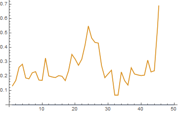
The problem with the nonstationarity of the out-of-sample estimated portfolio values is not mitigated by adding more in-sample data points and re-estimating the cointegrating vector(s):
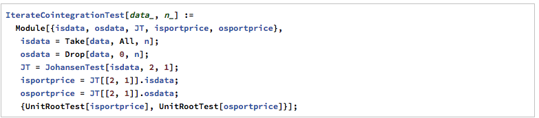
We continue to add more in-sample data points, reducing the size of the out-of-sample dataset correspondingly. But none of the tests for any of the out-of-sample datasets is able to reject the null hypothesis of a unit root in the portfolio price process: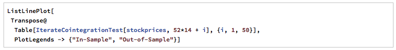
The Challenge of Cointegration Testing in Real Time
In our toy problem we know the out-of-sample prices of the constituent ETFs, and can therefore test the stationarity of the portfolio process out of sample. In a real world application, that discovery could only be made in real time, when the unknown, future ETFs prices are formed. In that scenario, all the researcher has to go on are the results of in-sample cointegration analysis, which demonstrate that the first cointegrating vector consistently yields a portfolio price process that is very likely stationary in sample (with high probability).
The researcher might understandably be persuaded, wrongly, that the same is likely to hold true in future. Only when the assumed cointegration relationship falls apart in real time will the researcher then discover that it’s not true, incurring significant losses in the process, assuming the research has been translated into some kind of trading strategy.
A great many analysts have been down exactly this path, learning this important lesson the hard way. Nor do additional “safety checks” such as, for example, also requiring high levels of correlation between the constituent processes add much value. They might offer the researcher comfort that a “belt and braces” approach is more likely to succeed, but in my experience it is not the case: the problem of non-stationarity in the out of sample price process persists.
Conclusion: Why Cointegration Breaks Down
We have seen how a portfolio of ETFs consistently estimated to be cointegrated in-sample, turns out to be non-stationary when tested out-of-sample. This goes to the issue of the low power of cointegration test, and their inability to estimate cointegrating vectors with sufficient accuracy. Analysts relying on standard tests such as the Johansen procedure to design their statistical arbitrage strategies are likely to be disappointed by the regularity with which their strategies break down in live trading.