
The research in this post and the related paper on Range Based EGARCH Option pricing Models is focused on the innovative range-based volatility models introduced in Alizadeh, Brandt, and Diebold (2002) (hereafter ABD). We develop new option pricing models using multi-factor diffusion approximations couched within this theoretical framework and examine their properties in comparison with the traditional Black-Scholes model.
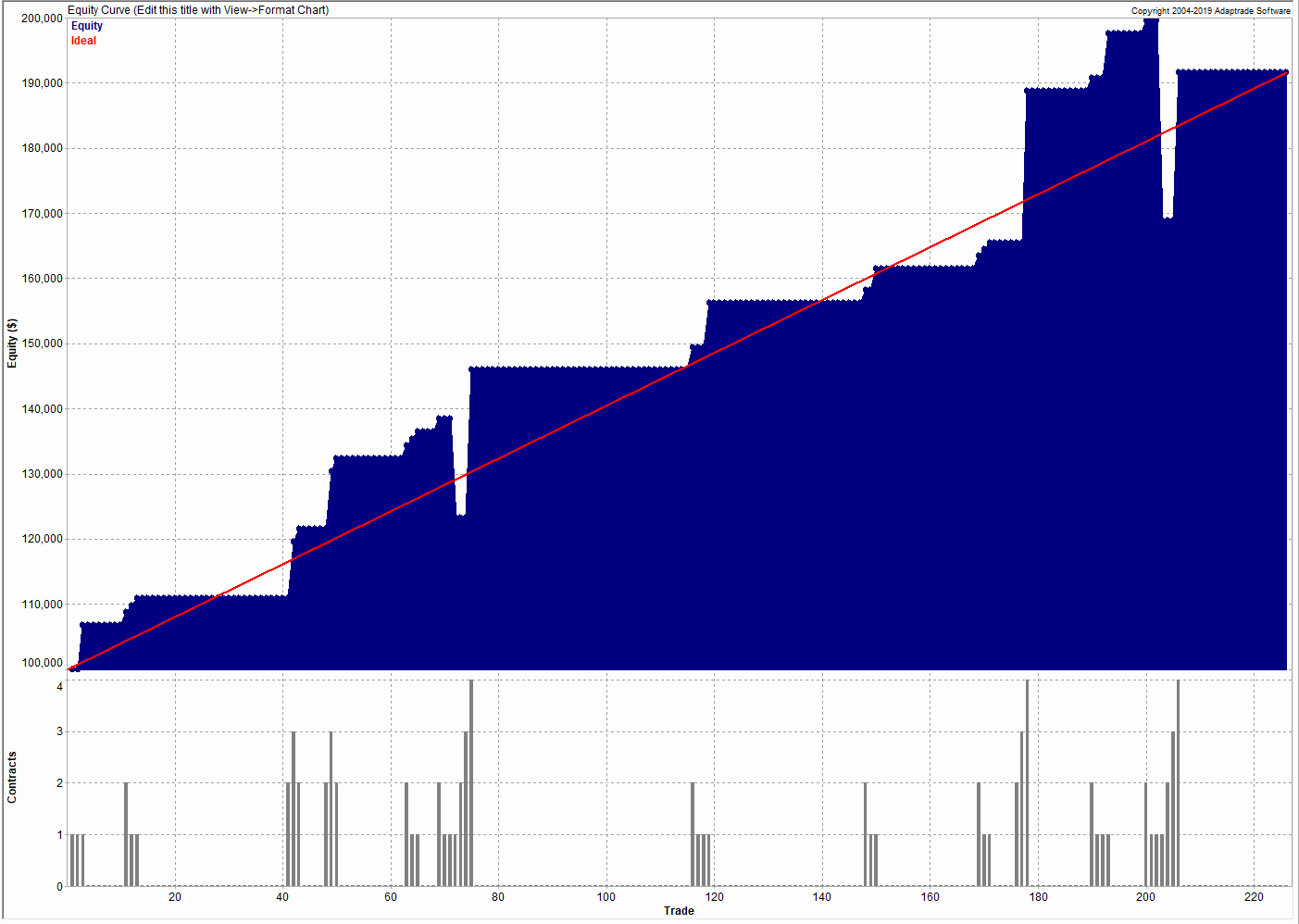
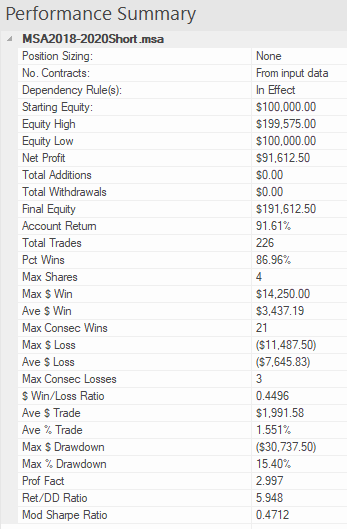
The two-factor version of the model, which I have applied successfully in various option arbitrage strategies, encapsulates the intuively appealing idea of a trending long term mean volatility process, around which oscillates a mean-reverting, transient volatility process. The option pricing model also incorporates asymmetry/leverage effects and well as correlation effects between the asset return and volatility processes, which results in a volatility skew.
The core concept behind Range-Based Exponential GARCH model is Log-Range estimator discussed in an earlier post on volatility metrics, which contains a lengthy exposition of various volatility estimators and their properties. (Incidentally, for those of you who requested a copy of my paper on Estimating Historical Volatility, I have updated the post to include a link to the pdf).

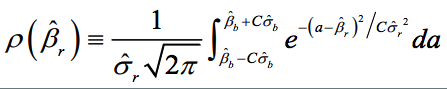
We assume that the log stock price s follows a drift-less Brownian motion ds = sdW. The volatility of daily log returns, denoted h= s/sqrt(252), is assumed constant within each day, at ht from the beginning to the end of day t, but is allowed to change from one day to the next, from ht at the end of day t to ht+1 at the beginning of day t+1. Under these assumptions, ABD show that the log range, defined as:
![]()
is to a very good approximation distributed as
![]()
where N[m; v] denotes a Gaussian distribution with mean m and variance v. The above equation demonstrates that the log range is a noisy linear proxy of log volatility ln ht. By contrast, according to the results of Alizadeh, Brandt,and Diebold (2002), the log absolute return has a mean of 0.64 + ln ht and a variance of 1.11. However, the distribution of the log absolute return is far from Gaussian. The fact that both the log range and the log absolute return are linear log volatility proxies (with the same loading of one), but that the standard deviation of the log range is about one-quarter of the standard deviation of the log absolute return, makes clear that the range is a much more informative volatility proxy. It also makes sense of the finding of Andersen and Bollerslev (1998) that the daily range has approximately the same informational content as sampling intra-daily returns every four hours.
Except for the model of Chou (2001), GARCH-type volatility models rely on squared or absolute returns (which have the same information content) to capture variation in the conditional volatility ht. Since the range is a more informative volatility proxy, it makes sense to consider range-based GARCH models, in which the range is used in place of squared or absolute returns to capture variation in the conditional volatility. This is particularly true for the EGARCH framework of Nelson (1990), which describes the dynamics of log volatility (of which the log range is a linear proxy).
ABD consider variants of the EGARCH framework introduced by Nelson (1990). In general, an EGARCH(1,1) model performs comparably to the GARCH(1,1) model of Bollerslev (1987). However, for stock indices the in-sample evidence reported by Hentschel (1995) and the forecasting performance presented by Pagan and Schwert (1990) show a slight superiority of the EGARCH specification. One reason for this superiority is that EGARCH models can accommodate asymmetric volatility (often called the “leverage effect,” which refers to one of the explanations of asymmetric volatility), where increases in volatility are associated more often with large negative returns than with equally large positive returns.
The one-factor range-based model (REGARCH 1) takes the form:
![]()
where the returns process Rt is conditionally Gaussian: Rt ~ N[0, ht2]
and the process innovation is defined as the standardized deviation of the log range from its expected value:
![]()
Following Engle and Lee (1999), ABD also consider multi-factor volatility models. In particular, for a two-factor range-based EGARCH model (REGARCH2), the conditional volatility dynamics) are as follows:
![]()
and
![]()
where ln qt can be interpreted as a slowly-moving stochastic mean around which log volatility ln ht makes large but transient deviations (with a process determined by the parameters kh, fh and dh).
The parameters q, kq, fq and dq determine the long-run mean, sensitivity of the long run mean to lagged absolute returns, and the asymmetry of absolute return sensitivity respectively.
The intuition is that when the lagged absolute return is large (small) relative to the lagged level of volatility, volatility is likely to have experienced a positive (negative) innovation. Unfortunately, as we explained above, the absolute return is a rather noisy proxy of volatility, suggesting that a substantial part of the volatility variation in GARCH-type models is driven by proxy noise as opposed to true information about volatility. In other words, the noise in the volatility proxy introduces noise in the implied volatility process. In a volatility forecasting context, this noise in the implied volatility process deteriorates the quality of the forecasts through less precise parameter estimates and, more importantly, through less precise estimates of the current level of volatility to which the forecasts are anchored.
read more…


