Algorithmic Trading Archives - Page 4 of 4 - QUANTITATIVE RESEARCH AND TRADING

February 5, 2019February 5, 2019

Daytrading Volatility ETFs

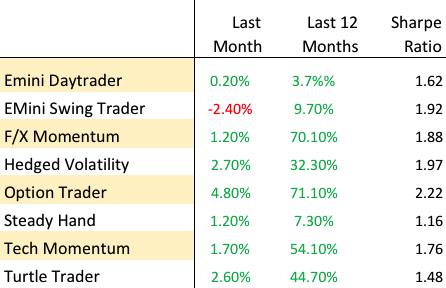
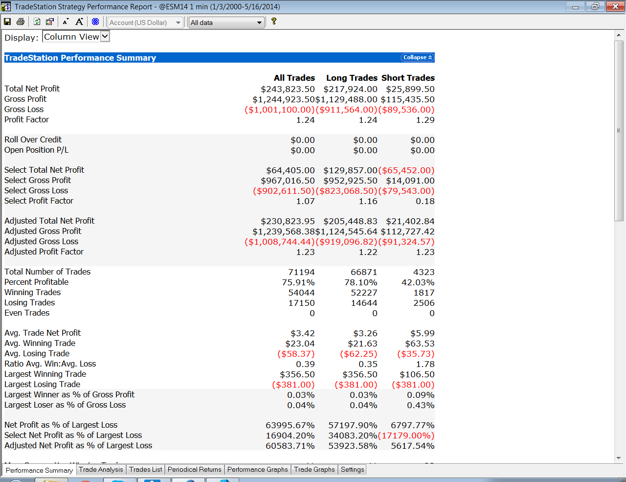
As we have discussed before, there is no standard definition of high frequency trading. For some, trading more than once or twice a day constitutes high frequency, while others regard anything less than several hundred times a session as low, or medium frequency trading. Hence in this post I have referred to “daytrading” since we can at least agree on that description for a strategy that exits all positions by the close of the session.

HFT Trading in ETFs – Challenges and Opportunities

High frequency trading in equities and ETFs offer their own opportunities and challenges compared to futures. Amongst the opportunities we might list:

Arbitrage between destinations (exchanges, dark pools) where the stock is traded
Earning rebates from the exchanges willing to pay for order flow
Arbitraging news flows amongst pairs or baskets of equities

When it comes to ETFs, unfortunately, the set of possibilities is more restricted than for single names and one is often obliged to dig deeply into the basket/replication/cointegration type of approach, which can be very challenging in a high frequency context. The risk of one leg of a multi-asset trade being left unfilled is such that one has to be willing to cross the spread to get the trade on. Depending on the trading platform and the quality of the execution algorithms, this can make trading the strategy prohibitively expensive.

In that case you have a number of possibilities to consider. You can simplify the trade, limit the number of stocks in the basket and hope that there is enough alpha left in the reduced strategy. You can focus on managing the trade execution sufficiently well that aggressive trading becomes necessary on relatively few occasions and you look to minimize the costs of paying the spread when they arise. You can design strategies with higher profit factors that are able to withstand the performance drag entailed in trading aggressively. Or you can design slower versions of the strategy where latency, fill rates and execution costs are not such critical factors.

Developing high frequency strategies in the volatility ETFs presents special challenges. Being fairly new, the products have limited histories, which makes modeling more of a challenge. One way to address this is to create synthetic series priced from the VIX futures, using the published methodology for constructing the ETFs. Be warned, though, that these synthetic series are likely to inflate your backtest results since they aren’t traded instruments.

Another practical problem that crops up regularly in products like UVXY and VXX is that the broker has difficulty locating stock for short selling. So you are limited to taking the strategy offline when that occurs, designing strategies that trade long only, or as we do, switching to other products when the ETF is unavailable to short.

Then there is the capacity issue. Despite their fast-growing popularity, volatility ETF funds are in many cases quite small, totaling perhaps a few hundred millions of dollars in AUM. You are never going to be able to construct a strategy capable of absorbing billions of dollars of investment in the ETF products alone.

Volatility and Alpha

For these reasons, volatility ETFs are not a natural choice for many investment strategists. But they do have one great advantage compared to other products: volatility. Volatility implies uncertainty about the true value of a security, which means that market participants can have very different views about what it is worth at any moment in time. So the prospects for achieving competitive advantage through superior analytical methods is much greater than for a stock that hardly moves at all and on whose value everyone concurs. Furthermore, volatility creates regular opportunities for hitting stops, and creating mini crashes or short squeezes, in which the security is temporarily under- or over-valued. If ever there was a security offering the potential for generating alpha, it is the volatility ETF.

The volatility of the VIX ETFs is enormous, by the standards of regular stocks. A typical stock might have an annual volatility of 30% to 60%. The lowest level ever seen in the VVIX index series so far is 70%. To give you an idea of how extreme it can become, during the latest market swoon in August the VVIX, the volatility-of-volatility for the S&P500 index, reached over 200% a year.

A Daytrading Strategy in the VXX

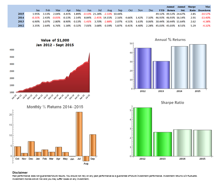
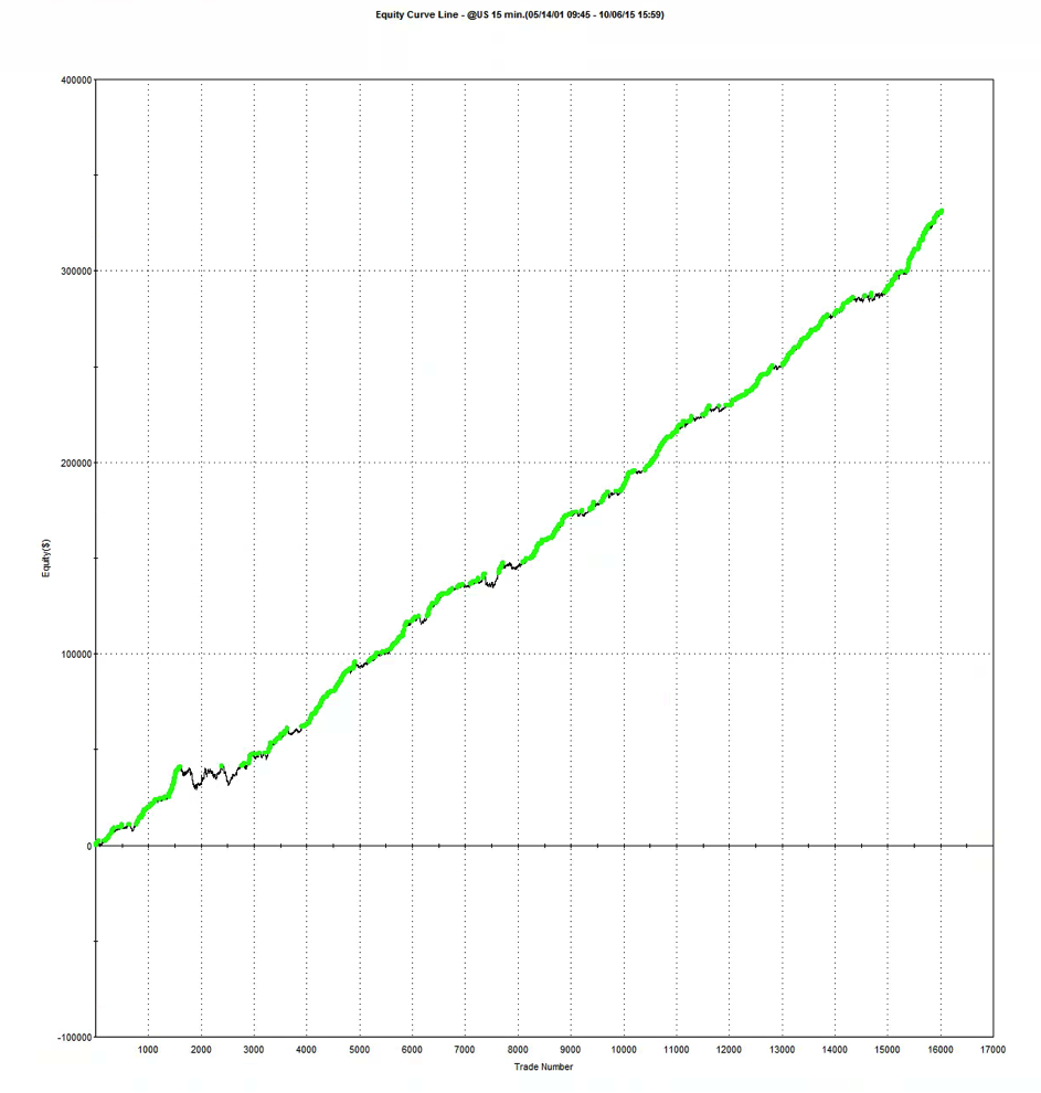
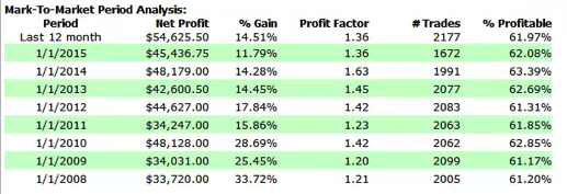
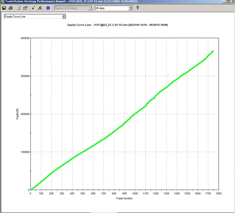
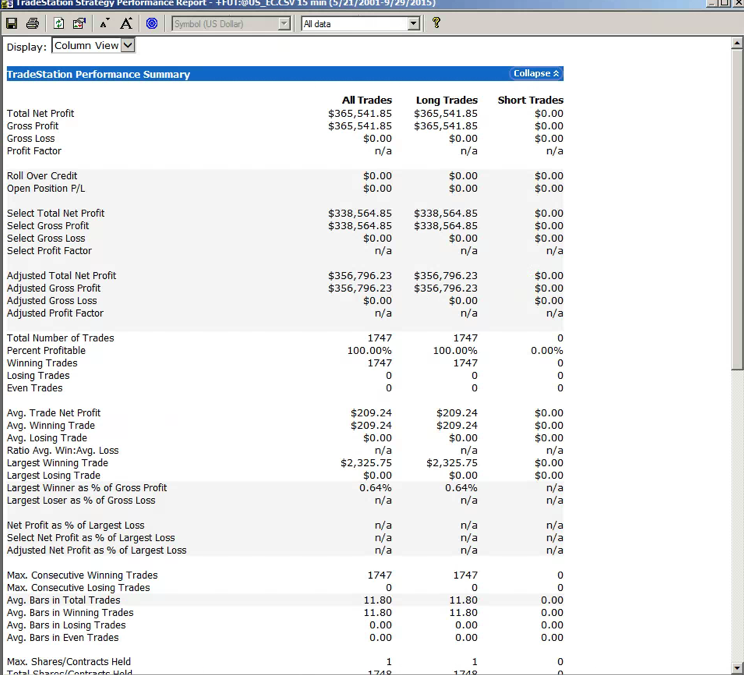
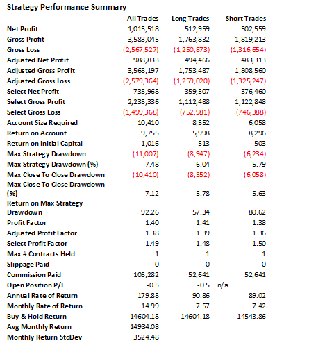
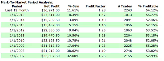
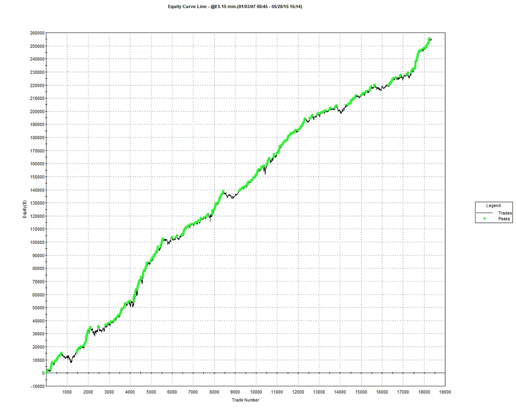
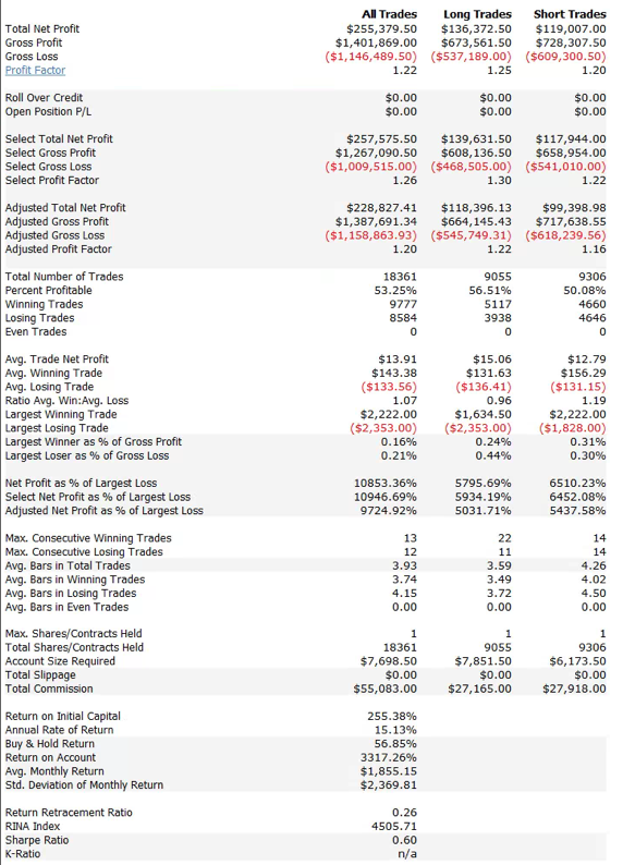
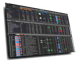
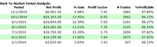
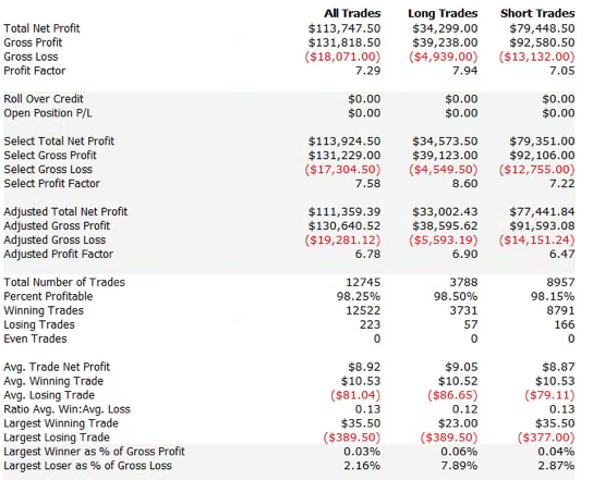
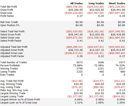
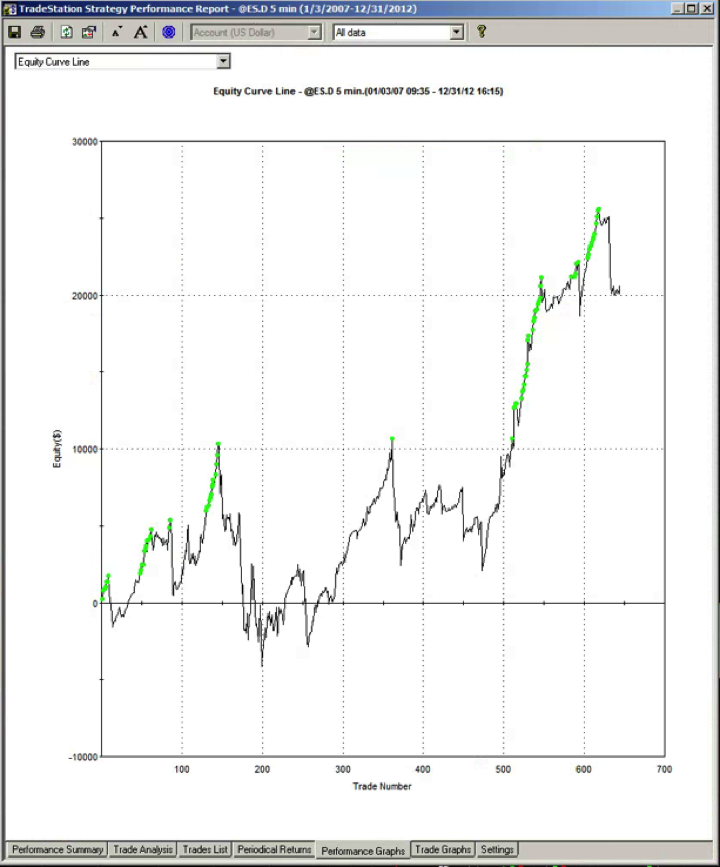
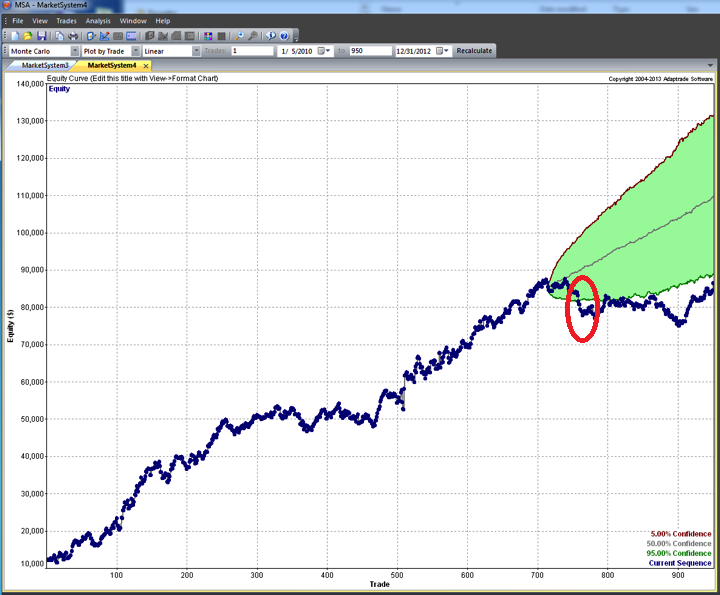
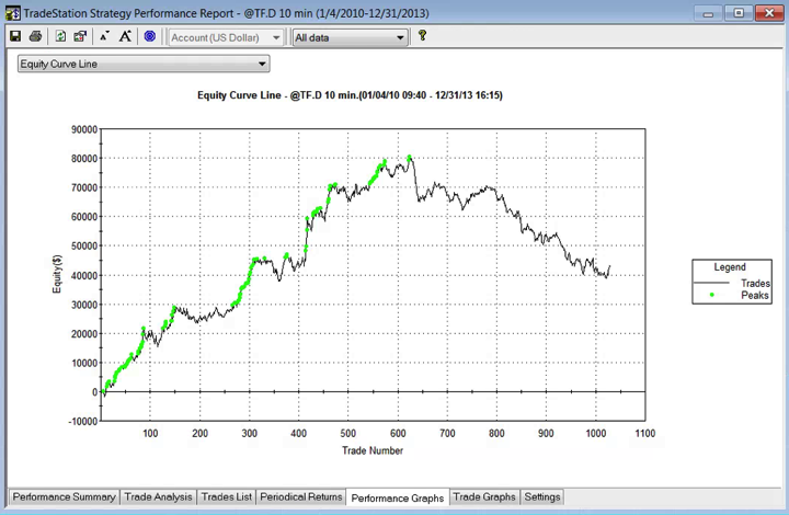
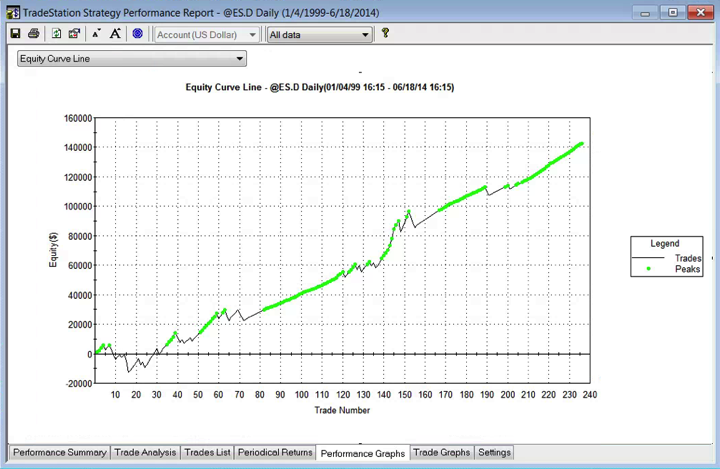
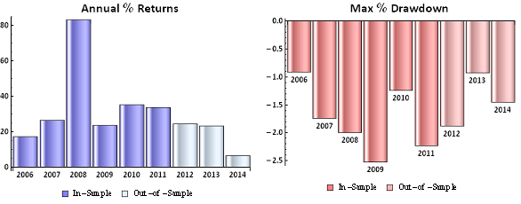
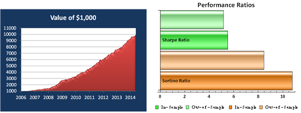
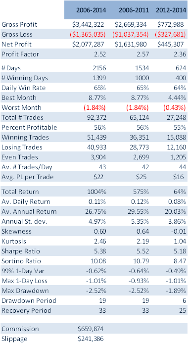
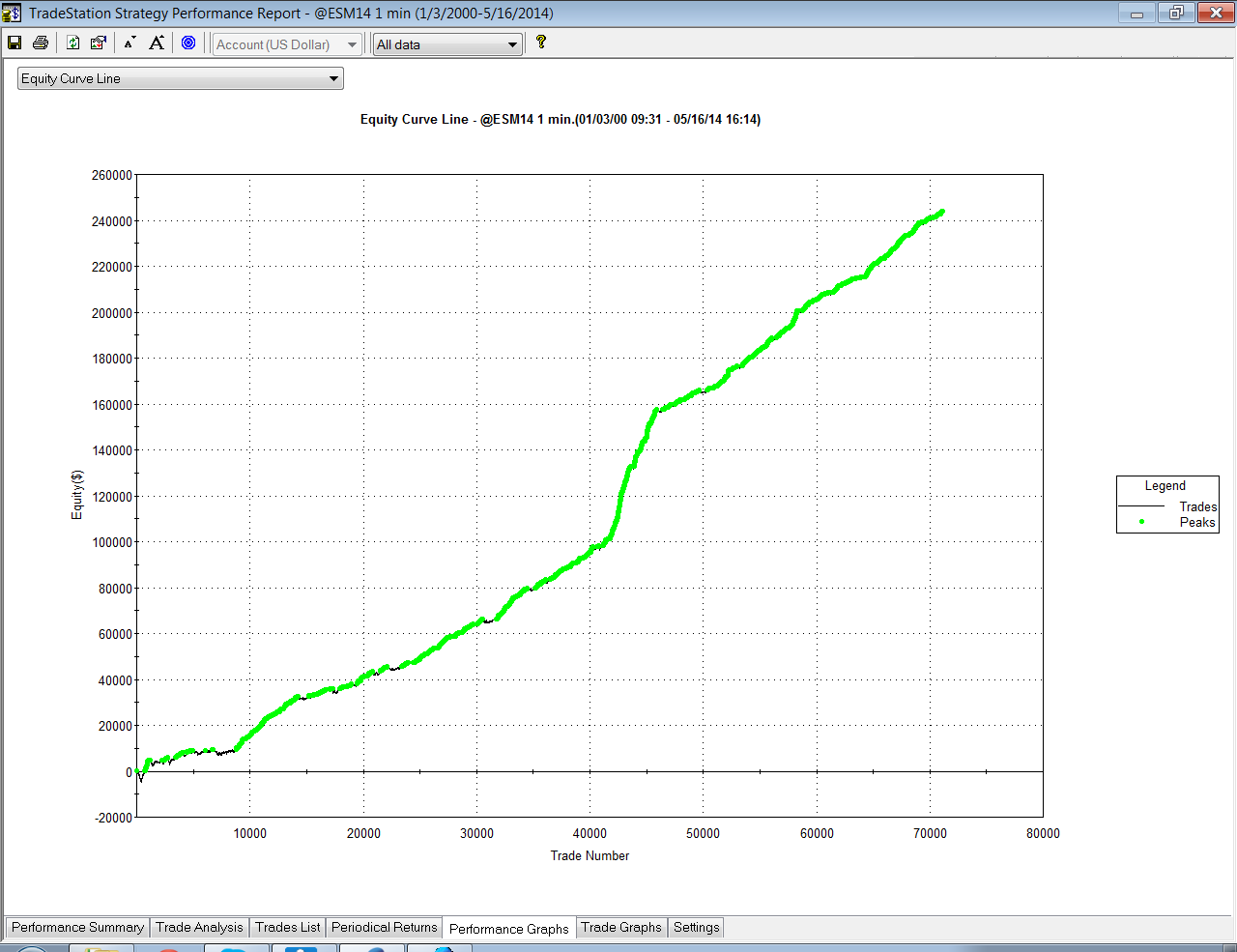
So, despite the challenges and difficulties, there are very good reasons to make the attempt to develop strategies for the volatility ETF products. My firm, Systematic Strategies, has developed several such algorithms that are combined to create a strategy that trades the volatility ETFs very successfully. Until recently, however, all of the sub-strategies we employ were longer term in nature, and entailed holding positions overnight. We wanted to develop higher frequency algorithms that could react more quickly to changes in the volatility landscape. We had to dig pretty deep into the arsenal of trading ideas to get there, but eventually we succeeded. After six months of live trading we were ready to release the new VXX daytrading algorithm into production for our volatility ETF strategy investors. Here’s how it looks (results are for a $100,000 account).

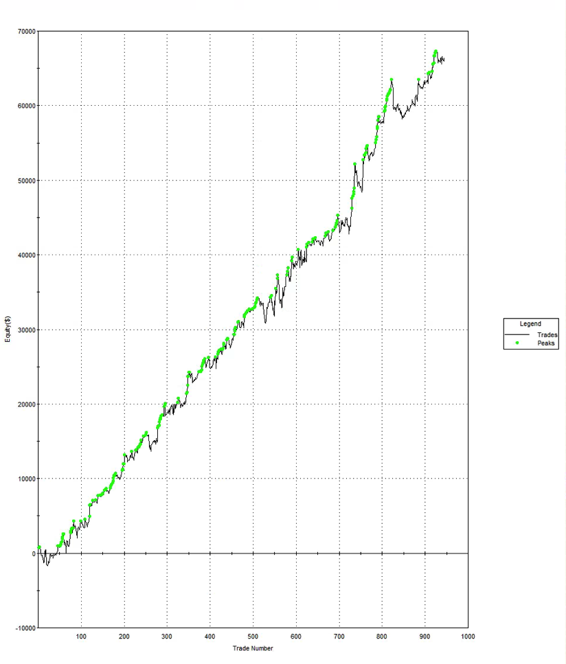
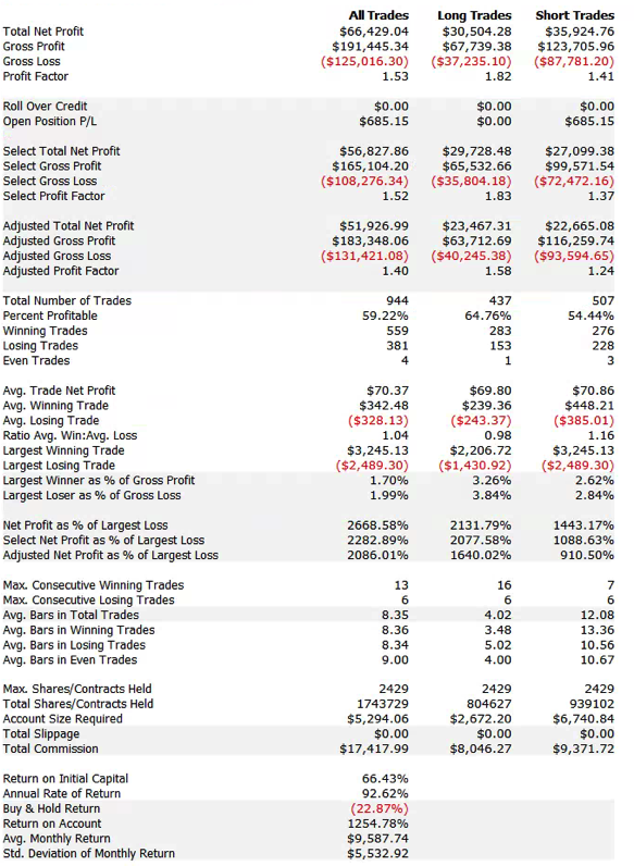
As you can see, the strategy trades up to around 10 times a day with a reasonable profit factor (1.53) and win rate of just under 60%. By itself, the strategy has a Sharpe Ratio of around 6, so it is well worth trading on its own. But its real value (for us) emerges when it is combined in appropriate proportion with the other, lower frequency algorithms in the volatility strategy. The additional alpha from the VXX strategy reduces the size of the loss in August and produces a substantial gain in September, taking the YTD return to just under 50%. Returns for Oct MTD are already at 16%.

January 29, 2019

Improving Trading System Performance Using a Meta-Strategy

What is a Meta-Strategy?

In my previous post on identifying drivers of strategy performance I mentioned the possibility of developing a meta-strategy.

A meta-strategy is a trading system that trades trading systems. The idea is to develop a strategy that will make sensible decisions about when to trade a specific system, in a way that yields superior performance compared to simply following the underlying trading system. Put another way, the simplest kind of meta-strategy is a long-only strategy that takes positions in some underlying trading system. At times, it will follow the underlying system exactly; at other times it is out of the market and ignore the trading system’s recommendations.

More generally, a meta-strategy can determine the size in which one, or several, systems should be traded at any point in time, including periods where the size can be zero (i.e. the system is not currently traded). Typically, a meta-strategy is long-only: in theory there is nothing to stop you developing a meta-strategy that shorts your underlying strategy from time to time, but that is a little counter-intuitive to say the least!

A meta-strategy is something that could be very useful for a fund-of-funds, as a way of deciding how to allocate capital amongst managers.

Caissa Capital operated a meta-strategy in its option arbitrage hedge fund back in the early 2000’s. The meta-strategy (we called it a “model management system”) selected from a half dozen different volatility models to be used for option pricing, depending their performance, as measured by around 30 different criteria. The criteria included both statistical metrics, such as the mean absolute percentage error in the forward volatility forecasts, as well as trading performance criteria such as the moving average of the trade PNL. The model management system probably added 100 – 200 basis points per annum to the performance the underlying strategy, so it was a valuable add-on.

Illustration of a Meta-Strategy in US Bond Futures

To illustrate the concept we will use an underlying system that trades US Bond futures at 15-minute bar intervals. The performance of the system is summarized in the chart and table below.

Strategy performance has been very consistent over the last seven years, in terms of the annual returns, number of trades and % win rate. Can it be improved further?

To assess this possibility we create a new data series comprising the points of the equity curve illustrated above. More specifically, we form a series comprising the open, high, low and close values of the strategy equity, for each trade. We will proceed to treat this as a new data series and apply a range of different modeling techniques to see if we can develop a trading strategy, in exactly the same way as we would if the underlying was a price series for a stock.

It is important to note here that, for the meta-strategy at least, we are working in trade-time, not calendar time. The x-axis will measure the trade number of the underlying strategy, rather than the date of entry (or exit) of the underlying trade. Thus equally spaced points on the x-axis represent different lengths of calendar time, depending on the duration of each trade.

It is necessary to work in trade time rather than calendar time because, unlike a stock, it isn’t possible to trade the underlying strategy whenever we want to – we can only enter or exit the strategy at points in time when it is about to take a trade, by accepting that trade or passing on it (we ignore the other possibility which is sizing the underlying trade, for now).

Another question is what kinds of trading ideas do we want to consider for the meta-strategy? In principle one could incorporate almost any trading concept, including the usual range of technical indictors such as RSI, or Bollinger bands. One can go further an use machine learning techniques, including Neural Networks, Random Forest, or SVM.

In practice, one tends to gravitate towards the simpler kinds of trading algorithm, such as moving averages (or MA crossover techniques), although there is nothing to say that more complex trading rules should not be considered. The development process follows a familiar path: you create a hypothesis, for example, that the equity curve of the underlying bond futures strategy tends to be mean-reverting, and then proceed to test it using various signals – perhaps a moving average, in this case. If the signal results in a potential improvement in the performance of the default meta-strategy (which is to take every trade in the underlying system system), one includes it in the library of signals that may ultimately be combined to create the finished meta-strategy.

As with any strategy development you should follows the usual procedure of separating the trade data to create a set used for in-sample modeling and out-of-sample performance testing.

Following this general procedure I arrived at the following meta-strategy for the bond futures trading system.

The modeling procedure for the meta-strategy has succeeded in eliminating all of the losing trades in the underlying bond futures system, during both in-sample and out-of-sample periods (comprising the most recent 20% of trades).

In general, it is unlikely that one can hope to improve the performance of the underlying strategy quite as much as this, of course. But it may well be possible to eliminate a sufficient proportion of losing trades to reduce the equity curve drawdown and/or increase the overall Sharpe ratio by a significant amount.

A Challenge / Opportunity

If you like the meta-strategy concept, but are unsure how to proceed, I may be able to help.

Send me the data for your existing strategy (see details below) and I will attempt to model a meta-strategy and send you the results. We can together evaluate to what extent I have been successful in improving the performance of the underlying strategy.

Here are the details of what you need to do:

1. You must have an existing, profitable strategy, with sufficient performance history (either real, simulated, or a mixture of the two). I don’t need to know the details of the underlying strategy, or even what it is trading, although it would be helpful to have that information.

2. You must send the complete history of the equity curve of the underlying strategy, in Excel format, with column headings Date, Open, High, Low, Close. Each row represents consecutive trades of the underlying system and the O/H/L/C refers to the value of the equity curve for each trade.

3. The history must comprise at least 500 trades as an absolute minimum and preferably 1000 trades, or more.

4. At this stage I can only consider a single underlying strategy (i.e. a single equity curve)

5. You should not include any software or algorithms of any kind. Nothing proprietary, in other words.

6. I will give preference to strategies that have a (partial) live track record.

As my time is very limited these days I will not be able to deal with any submissions that fail to meet these specifications, or to enter into general discussions about the trading strategy with you.

You can reach me at jkinlay@systematic-strategies.com

December 4, 2018

High Frequency Trading Strategies

Most investors have probably never seen the P&L of a high frequency trading strategy. There is a reason for that, of course: given the typical performance characteristics of a HFT strategy, a trading firm has little need for outside capital. Besides, HFT strategies can be capacity constrained, a major consideration for institutional investors. So it is amusing to see the reaction of an investor on encountering the track record of a HFT strategy for the first time. Accustomed as they are to seeing Sharpe ratios in the range of 0.5-1.5, or perhaps as high as 1.8, if they are lucky, the staggering risk-adjusted returns of a HFT strategy, which often have double-digit Sharpe ratios, are truly mind-boggling.

By way of illustration I have attached below the performance record of one such HFT strategy, which trades around 100 times a day in the eMini S&P 500 contract (including the overnight session). Note that the edge is not that great – averaging 55% profitable trades and profit per contract of around half a tick – these are some of the defining characteristics of HFT trading strategies. But due to the large number of trades it results in very substantial profits. At this frequency, trading commissions are very low, typically under $0.1 per contract, compared to $1 – $2 per contract for a retail trader (in fact an HFT firm would typically own or lease exchange seats to minimize such costs).

Hidden from view in the above analysis are the overhead costs associated with implementing such a strategy: the market data feed, execution platform and connectivity capable of handling huge volumes of messages, as well as algo logic to monitor microstructure signals and manage order-book priority. Without these, the strategy would be impossible to implement profitably.

Scaling things back a little, lets take a look at a day-trading strategy that trades only around 10 times a day, on 15-minute bars. Although not ultra-high frequency, the strategy nonetheless is sufficiently high frequency to be very latency sensitive. In other words, you would not want to try to implement such a strategy without a high quality market data feed and low-latency trading platform capable of executing at the 1-millisecond level. It might just be possible to implement a strategy of this kind using TT’s ADL platform, for example.

While the win rate and profit factor are similar to the first strategy, the lower trade frequency allows for a higher trade PL of just over 1 tick, while the equity curve is a lot less smooth reflecting a Sharpe ratio that is “only” around 2.7.

The critical assumption in any HFT strategy is the fill rate. HFT strategies execute using limit or IOC orders and only a certain percentage of these will ever be filled. Assuming there is alpha in the signal, the P&L grows in direct proportion to the number of trades, which in turn depends on the fill rate. A fill rate of 10% to 20% is usually enough to guarantee profitability (depending on the quality of the signal). A low fill rate, such as would typically be seen if one attempted to trade on a retail trading platform, would destroy the profitability of any HFT strategy.

To illustrate this point, we can take a look at the outcome if the above strategy was implemented on a trading platform which resulted in orders being filled only when the market trades through the limit price. It isn’t a pretty sight.

The moral of the story is: developing a HFT trading algorithm that contains a viable alpha signal is only half the picture. The trading infrastructure used to implement such a strategy is no less critical. Which is why HFT firms spend tens, or hundreds of millions of dollars developing the best infrastructure they can afford.

October 16, 2018

Algorithmic Trading

MOVING FROM RESEARCH TO TRADING

I have written recently about the comparative advantages of different programming languages in the context of research and trading (see here). My sense of it is that there is no single “ideal” programming language – the best strategy is to pick an appropriate tool for the job and there are usually several reasonable choices one could make.

If you are engaged in econometrics research, you might choose a package like RATS, Eviews, Gauss, or Prof. James Davidson’s excellent and inexpensive TSM, which I have used for many years and can recommend highly. For a latency-sensitive high frequency trading application, you will probably want to use something like C++, or possibly a 3rd party algo system like Apama or Tethys. But for algorithmic trading systems of intermediate frequency the choice appears almost unlimited.

The problem with retail trading tools like TradeStation, Multicharts, or Amibroker, is that they are designed primarily for single-asset strategies. That may be ok for futures trading,where more often than not the focus is on a single underlying, but in equities the opposite is true. Using one of these products to develop and implement a pairs trading strategy is a stretch. As for portfolio analytics – forget it.

This is where more general, high level languages like R, Matlab or Mathematica come in: their greater power and flexibility is handling large, multivariate data sets makes it much more straightforward to develop portfolio strategies. And they can often bridge the gap between R&D and implementation quite easily: code that was used in the research stage can often be quickly re-tooled to work in a production version of the system. As for production systems, there is now a significant cottage industry of traders who use Matlab in algo trading. R has a similar following (see here).

In addition to parallelizing the code (for use with the Parallel Computing Toolbox) to speed up the research phase, you might also want to implement a hybrid system by re-coding the slower routines in C++, to create a mex file (for details see here). Matlab’s Profiler is a useful tool for identifying code bottlenecks. In a recent piece of research in which I was evaluating over 30,000,000 cointegrated portfolios, I discovered to my surprise that the main code bottleneck was the multiple calls to Matlab’s std function, a problem easily fixed with a few lines of C++ code. The resulting hybrid program executed at more than twice the speed – important when your run time might be several hours, or even days.

HOOKING UP THE EXECUTION PLATFORM

The main challenge for developers using generic tools like Mathematica, Matlab or R is the implementation stage of the project. Providing connectivity to brokerage/execution platforms never seemed high on the list of priorities for Wolfram or Mathworks and things are similarly hit or miss with R.

Belatedly, Mathematica now offers a link to Bloomberg via its Finance Platform. Matlab, meanwhile, offers a Trading Toolbox, which supposedly offers connectivity , not only to Bloomberg, but also Interactive Brokers and Trading Technologies, amongst other platforms. Unfortunately, the toolbox interface to IB appears to rely on outdated 1990s ActiveX technology, which is flakey at best. In tests, I was unable to make progress past the ‘not connected’ error message.

At that point I turned to Yair Altman’s IB-Matlab product. Happily, this uses IB’s Java api, which is a great deal more robust than the ActiveX platform. It’s been some time since I last used IB-Matlab and was pleased to see that Yair has been very busy over the intervening period, building the capabilities of the system and providing very comprehensive documentation for it. With Yair’s help, it took me no time at all to get up and running and within a day or two the system was executing orders flawlessly in IB’s TWS. The relatively few snags I ran into were almost all due to IB’s extremely terse error messaging, which often gives almost no clue as to what the issue might be. Fortunately, Yair is very generous with his time in providing support to his users and his responses to me questions were fast and detailed.

EXECUTION ALGOS

With intermediate systems trading at frequencies of, say, 5-minutes to daily, one has a choice to make as regards execution. Given that the strategy is not very latency sensitive, it is certainly conceivable to develop one’s own execution algos in Matlab. However, platforms like TWS are equipped with native algos, not only from IB, but also other providers like Credit Suisse and Jeffries.

Actually, I have found several of IB’s own algos such as Scaletrader and Accumulate/Distribute to be very effective. Certainly IB seems very proud of them – IB CEO Thomas Peterffy has patented at least one of them. Accumulate/Distribute, for instance, is quite sophisticated, allowing the user to randomize and slice the size and interval between individual orders, use passive or aggressive order types, and pause execution on a news alert, or when the price falls below a moving average, or outside a specified range.

There is much to be said for using algos native to the execution platform rather than reinventing the wheel, providing the cost is reasonable. So, while it is perfectly feasible to build execution algos in Matlab, it typically isn’t necessary – in most cases standard algos will suffice.

There are exceptions, of course. IB doesn’t offer the kind of basket-trading capabilities that are available in advanced algo platforms like Tethys or RediPlus. In those systems, for example, you can set the level of long/short imbalance in the portfolio that you are willing to tolerate and the algo will speed up or slow down execution of trades in individual components of the basket to maintain the dollar imbalance within that tolerance. You can also manage the sector risk dynamically during execution.

Those kind of advanced capabilities don’t come cheap and you wont find them at IB, or any other retail platform. If you need that kind of functionality, for example, because you are trading a long/short equity portfolio within a universe of 200-300 names, your best option is probably to switch to a different execution platform. Otherwise you will need to code a custom algo in your language of choice.

For many quantitative strategies, (at least the low frequency ones) IB’s standard algos are often good enough. The Accumulate/Distribute algo, for instance, will show a visual representation of the progress of the execution of individuals legs of a pairs trade, and it is easy enough to identify a potential imbalance and adjust the algo parameters in real time. If you are only trading pairs, or small portfolios of cointegrated securities, it probably isn’t worthwhile to develop the sophisticated logic that would be required to handle the adjustment of the execution of individual legs of a trade in a fully automated way. A large portfolio would be a different matter, however.

MATLAB EXAMPLE

I thought it might be instructive to take a look at how you might implement the execution of a strategy in Matlab, using IB algos. In the Matlab code fragment below, the (2 x nTickers) array tradeActions contains, in the first row, the action we wish to take (1 = BUY, -1 = SELL, -2 = SELL SHORT) and in the second row the (absolute value of) the number of shares we wish to trade for tickers i =1:nTickers. We break each order up into hundred lots and odd lots, routing the former via IB’s Accumulate/Distribute algo and the latter as passive REL orders (note that A/D will typically randomize the timing of each sub-order, while REL orders are posted directly into the market). The Matlab function AccumulateDistribute implements the most important features of IB’s A/D algo, including random size and time slicing of the order. Orders are submitted as passive REL orders with zero offset (so they will sit on the current bid or ask) – obviously you would typically want to consider allowing some non-zero offset for less liquid securities. It is not hard to envisage how one might further enhance the algo to monitor the progress of the execution and speed up or slow down certain orders accordingly.

A couple of IB api “gotchas” to be aware of:

(i) IB requires unique and monotonically increasing orderIds for each order. One way to do this, suggested by Yair, is to use orderId = round((now-735000)*3e5); This fails when you are submitting a number of orders sequentially at high speed (say in a for loop), where the time increments are sub-second, so you need to pass the orderID back and force a minimal increment, as I have in the code below.

(ii) It is very important to specify the primary exchange of each security: securities with identical tickers can be found trading on different exchanges. Failing to specify the primary exchange in such a case will result in IB rejecting the order with a typically cryptic api message.

Continue reading “Algorithmic Trading”

October 2, 2018

A Comparison of Programming Languages

Towards the end of last year I wrote a post (see here) about the advent of modern programming languages, including the JIT compiled Julia and visual programming language ADL from Trading Technologies. My conclusion (based on a not very scientific sample) was that we appear to be at the tipping point, where the speed of newer, high level languages languages is approaching that of the fastest compiled languages like C/C++.

Now comes a formal academic study of the topic in A Comparison of Programming Languages in Economics, Aruoba and Fernandez-Villaverde, 2014. Using the neoclassical growth model, the authors conduct a benchmark test in C++11, Fortran 2008, Java, Julia, Python, Matlab, Mathematica, and R, implementing the same algorithm, value function
iteration with grid search, in each of the languages. They report the execution times of the codes in a Mac and in a Windows computer and briefly comment on the strengths and weaknesses of each language.

The conclusions from the study mirror my own thoughts on the subject very closely. The authors find that:

C++ and Fortran are still considerably faster than any other alternative, although one needs to be careful with the choice of compiler.
C++ compilers have advanced enough that, contrary to the situation in the 1990s and some folk wisdom, C++ code runs slightly faster (5-7 percent) than Fortran code.
Julia delivers outstanding performance. Execution speed is only between 2.64 and 2.70 times slower than the execution speed of the best C++ compiler.
Baseline Python was slow. Using the Pypy implementation, it runs around 44 times slower than in C++. Using the default CPython interpreter, the code runs between 155 and 269 times slower than in C++.
Matlab is between 9 to 11 times slower than the best C++ executable.
R runs between 475 to 491 times slower than C++. If the code is compiled, the code is between 243 to 282 times slower.
Hybrid programming and special approaches can deliver considerable speed ups. For example, when combined with Mex files, Matlab is only 1.24 to 1.64 times slower than C++ and when combined with Rcpp, R is between 3.66 and 5.41 times slower. Similar numbers hold for Numba (a just-in-time compiler for Python that uses decorators) and Cython (a static compiler for writing C extensions for Python) in the Python ecosystem.
Mathematica is only about three times slower than C++, but only after a considerable rewriting of the code to take advantage of the peculiarities of the language. The baseline version of the algorithm in Mathematica is considerably slower.

C++ still represents the benchmark for speed, but not by much. It is barely faster than the old stalwart, Fortran, and only 1.5 – 3 times faster than up-and-coming rivals amongst the higher level languages (especially when you allow for hybrid programming to speed up the slowest algorithms).

So, as regards developing financial models and trading systems, my questions are (as before):

Why would anyone prefer Python, given that there is a much faster, free alternative in Julia, which is just as easy a language to program in?
What justification is there for preferring R to Matlab, other than cost?
Why does anyone bother with Java? If speed is the critical issue, there are faster alternatives. If you like the relative simplicity of the syntax, Julia is cleaner, simpler and just as fast in execution.

When you reach a point where a high level language like Matlab is only around 1.5x – 2x slower than C++, you really have to question whether the latter is an appropriate choice. Yes, of course, in mission-critical applications where you need access to the hardware layer for speed purposes, C++ is the way to go. But for so many applications, that just isn’t the case.

What matters, far, far more, are the months of costly and laborious programming effort that is often required to reproduce basic functionality that is already embedded in higher level languages like Matlab or Mathematica. Not only that, but the end result of a C++ /Java development effort is likely to be notoriously inflexible by comparison. That’s a huge drawback. Rarely, if ever, does a piece of research translate flawlessly into production – it requires one to iterate towards a final solution, often making significant changes to the design of the system in the light of practical experience.

If I had to guess, based on my experience, I would say that 80% or more of development tasks in quantitative research and trading would produce a superior result if preference was given to using a higher level language for the initial development. When the system is sufficiently stable to put into production, you simply create a hybrid application by recoding any mission-critical components for which speed is an issue in C++.

Finally, where does that leave my beloved Mathematica? To be fair, while you don’t have the joys of strong typing to contend with, Mathematica’s syntax is just as demanding and uncompromising as C++ – a missed comma or incorrectly placed bracket is just as critical. But, the point is, while in C++ the syntactical rigor is just annoying, in Mathematica it’s worth putting up with because the productivity is so much greater. A competent programmer can produce, in a single line of Mathematica code, a program that would require hundreds, if not thousands of lines of C++ code to accomplish. Sure, he might get the syntax wrong at first: but it’s only a single line of code and the interactive gui interface makes debugging very simple.

That said, while Mathematica can be very tedious to use for procedural programming, it excels in three areas:

1. Symbolic programming. Anything involving mathematical symbols and equations – Mathematica is #1

2. User interface. In Mathematica, it is trivial to build a sophisticated, dynamic gui in no time at all, again, often in 1-2 lines of code

3. Functional programming. Anything that can be thought of as a function, Mathematica handles extremely well. We are not talking about finding a square root here: I mean extremely complex functions that, again, might take hundreds of lines of code in another language.

It is also worth pointing out that Mathematica comes supplied with functionality that Matlab provides only through numerous, costly add-on packages.

CONCLUSION
Before I allow a development team to start mindlessly coding up a system in Java or C++, I want to hear their reasons why they aren’t going to do it 10x faster in another, higher level language. “We always use C++/Java for production” is not a reason. Specifically, which parts of the system require the additional 1.5x speed-up, and why can’t they be coded as dlls (Matlab mex functions)?

Finally, on a cost-benefit basis, ask yourself how much you might benefit if the months and tens (or hundreds) of thousands of dollars wasted on developing in C++ were instead spent on researching and developing new trading ideas.

October 2, 2018October 2, 2018

Quant Strategies in 2018

Quant Strategies – Performance Summary Sept. 2018

The end of Q3 seems like an appropriate time for an across-the-piste review of how systematic strategies are performing in 2018. I’m using the dozen or more strategies running on the Systematic Algotrading Platform as the basis for the performance review, although results will obviously vary according to the specifics of the strategy. All of the strategies are traded live and performance results are net of subscription fees, as well as slippage and brokerage commissions.

Volatility Strategies

Those waiting for the hammer to fall on option premium collecting strategies will have been disappointed with the way things have turned out so far in 2018. Yes, February saw a long-awaited and rather spectacular explosion in volatility which completely destroyed several major volatility funds, including the VelocityShares Daily Inverse VIX Short-Term ETN (XIV) as well as Chicago-based hedged fund LJM Partners (“our goal is to preserve as much capital as possible”), that got caught on the wrong side of the popular VIX carry trade. But the lack of follow-through has given many volatility strategies time to recover. Indeed, some are positively thriving now that elevated levels in the VIX have finally lifted option premiums from the bargain basement levels they were languishing at prior to February’s carnage. The Option Trader strategy is a stand-out in this regard: not only did the strategy produce exceptional returns during the February melt-down (+27.1%), the strategy has continued to outperform as the year has progressed and YTD returns now total a little over 69%. Nor is the strategy itself exceptionally volatility: the Sharpe ratio has remained consistently above 2 over several years.

Hedged Volatility Trading

Investors’ chief concern with strategies that rely on collecting option premiums is that eventually they may blow up. For those looking for a more nuanced approach to managing tail risk the Hedged Volatility strategy may be the way to go. Like many strategies in the volatility space the strategy looks to generate alpha by trading VIX ETF products; but unlike the great majority of competitor offerings, this strategy also uses ETF options to hedge tail risk exposure. While hedging costs certainly acts as a performance drag, the results over the last few years have been compelling: a CAGR of 52% with a Sharpe Ratio close to 2.

F/X Strategies

One of the common concerns for investors is how to diversify their investment portfolios, especially since the great majority of assets (and strategies) tend to exhibit significant positive correlation to equity indices these days. One of the characteristics we most appreciate about F/X strategies in general and the F/X Momentum strategy in particular is that its correlation to the equity markets over the last several years has been negligible. Other attractive features of the strategy include the exceptionally high win rate – over 90% – and the profit factor of 5.4, which makes life very comfortable for investors. After a moderate performance in 2017, the strategy has rebounded this year and is up 56% YTD, with a CAGR of 64.5% and Sharpe Ratio of 1.89.

Equity Long/Short

Thanks to the Fed’s accommodative stance, equity markets have been generally benign over the last decade to the benefit of most equity long-only and long-short strategies, including our equity long/short Turtle Trader strategy , which is up 31% YTD. This follows a spectacular 2017 (+66%) , and is in line with the 5-year CAGR of 39%. Notably, the correlation with the benchmark S&P500 Index is relatively low (0.16), while the Sharpe Ratio is a respectable 1.47.

Equity ETFs – Market Timing/Swing Trading

One alternative to the traditional equity long/short products is the Tech Momentum strategy. This is a swing trading strategy that exploits short term momentum signals to trade the ProShares UltraPro QQQ (TQQQ) and ProShares UltraPro Short QQQ (SQQQ) leveraged ETFs. The strategy is enjoying a banner year, up 57% YTD, with a four-year CAGR of 47.7% and Sharpe Ratio of 1.77. A standout feature of this equity strategy is its almost zero correlation with the S&P 500 Index. It is worth noting that this strategy also performed very well during the market decline in Feb, recording a gain of over 11% for the month.

Futures Strategies

It’s a little early to assess the performance of the various futures strategies in the Systematic Strategies portfolio, which were launched on the platform only a few months ago (despite being traded live for far longer). For what it is worth, both of the S&P 500 E-Mini strategies, the Daytrader and the Swing Trader, are now firmly in positive territory for 2018. Obviously we are keeping a watchful eye to see if the performance going forward remains in line with past results, but our experience of trading these strategies gives us cause for optimism.

Conclusion: Quant Strategies in 2018

There appear to be ample opportunities for investors in the quant sector across a wide range of asset classes. For investors with equity market exposure, we particularly like strategies with low market correlation that offer significant diversification benefits, such as the F/X Momentum and F/X Momentum strategies. For those investors seeking the highest risk adjusted return, option selling strategies like the Option Trader strategy are the best choice, while for more cautious investors concerned about tail risk the Hedged Volatility strategy offers the security of downside protection. Finally, there are several new strategies in equities and futures coming down the pike, several of which are already showing considerable promise. We will review the performance of these newer strategies at the end of the year.

Go here for more information about the Systematic Algotrading Platform.

September 23, 2018September 23, 2018

High Frequency Trading with ADL – JonathanKinlay.com

Trading Technologies’ ADL is a visual programming language designed specifically for trading strategy development that is integrated in the company’s flagship XTrader product. Despite the radically different programming philosophy, my experience of working with ADL has been delightfully easy and strategies that would typically take many months of coding in C++ have been up and running in a matter of days or weeks. An extract of one such strategy, a high frequency scalping trade in the E-Mini S&P 500 futures, is shown in the graphic above. The interface and visual language is so intuitive to a trading system developer that even someone who has never seen ADL before can quickly grasp at least some of what it happening in the code.

Strategy Development in Low vs. High-Level Languages
What are the benefits of using a high level language like ADL compared to programming languages like C++/C# or Java that are traditionally used for trading system development? The chief advantage is speed of development: I would say that ADL offers the potential up the development process by at least one order of magnitude. A complex trading system would otherwise take months or even years to code and test in C++ or Java, can be implemented successfully and put into production in a matter of weeks in ADL. In this regard, the advantage of speed of development is one shared by many high level languages, including, for example, Matlab, R and Mathematica. But in ADL’s case the advantage in terms of time to implementation is aided by the fact that, unlike generalist tools such as MatLab, etc, ADL is designed specifically for trading system development. The ADL development environment comes equipped with compiled pre-built blocks designed to accomplish many of the common tasks associated with any trading system such as acquiring market data and handling orders. Even complex spread trades can be developed extremely quickly due to the very comprehensive library of pre-built blocks.

Integrating Research and Development
One of the drawbacks of using a higher level language for building trading systems is that, being interpreted rather than compiled, they are simply too slow – one or more orders of magnitude, typically – to be suitable for high frequency trading. I will come on to discuss the execution speed issue a little later. For now, let me bring up a second major advantage of ADL relative to other high level languages, as I see it. One of the issues that plagues trading system development is the difficulty of communication between researchers, who understand financial markets well, but systems architecture and design rather less so, and developers, whose skill set lies in design and programming, but whose knowledge of markets can often be sketchy. These difficulties are heightened where researchers might be using a high level language and relying on developers to re-code their prototype system to get it into production. Developers typically (and understandably) demand a high degree of specificity about the requirement and if it’s not included in the spec it won’t be in the final deliverable. Unfortunately, developing a successful trading system is a highly non-linear process and a researcher will typically have to iterate around the core idea repeatedly until they find a combination of alpha signal and entry/exit logic that works. In other words, researchers need flexibility, whereas developers require specificity. ADL helps address this issue by providing a development environment that is at once highly flexible and at the same time powerful enough to meet the demands of high frequency trading in a production environment. It means that, in theory, researchers and developers can speak a common language and use a common tool throughout the R&D development cycle. This is likely to reduce the kind of misunderstanding between researchers and developers that commonly arise (often setting back the implementation schedule significantly when they do).

Latency
Of course, at least some of the theoretical benefit of using ADL depends on execution speed. The way the problem is typically addressed with systems developed in high level languages like Matlab or R is to recode the entire system in something like C++, or to recode some of the most critical elements and plug those back into the main Matlab program as dlls. The latter approach works, and preserves the most important benefits of working in both high and low level languages, but the resulting system is likely to be sub-optimal and can be difficult to maintain. The approach taken by Trading Technologies with ADL is very different. Firstly, the component blocks are written in C# and in compiled form should run about as fast as native code. Secondly, systems written in ADL can be deployed immediately on a co-located algo server that is plugged directly into the exchange, thereby reducing latency to an acceptable level. While this is unlikely to sufficient for an ultra-high frequency system operating on the sub-millisecond level, it will probably suffice for high frequency systems that operate at speeds above above a few millisecs, trading up to say, around 100 times a day.

Fill Rate and Toxic Flow
For those not familiar with the HFT territory, let me provide an example of why the issues of execution speed and latency are so important. Below is a simulated performance record for a HFT system in ES futures. The system is designed to enter and exit using limit orders and trades around 120 times a day, with over 98% profitability, if we assume a 100% fill rate. So far so good. But a 100% fill rate is clearly unrealistic. Let’s look at a pessimistic scenario: what if we got filled on orders only when the limit price was exceeded? (For those familiar with the jargon, we are assuming a high level of flow toxicity) The outcome is rather different: Neither scenario is particularly realistic, but the outcome is much more likely to be closer to the second scenario rather than the first if we our execution speed is slow, or if we are using a retail platform such as Interactive Brokers or Tradestation, with long latency wait times. The reason is simple: our orders will always arrive late and join the limit order book at the back of the queue. In most cases the orders ahead of ours will exhaust demand at the specified limit price and the market will trade away without filling our order. At other times the market will fill our order whenever there is a large flow against us (i.e. a surge of sell orders into our limit buy), i.e. when there is significant toxic flow. The proposition is that, using ADL and the its high-speed trading infrastructure, we can hope to avoid the latter outcome. While we will never come close to achieving a 100% fill rate, we may come close enough to offset the inevitable losses from toxic flow and produce a decent return. Whether ADL is capable of fulfilling that potential remains to be seen.

More on ADL
For more information on ADL go here.

September 11, 2018

How Not to Develop Trading Strategies – A Cautionary Tale

In his post on Multi-Market Techniques for Robust Trading Strategies (http://www.adaptrade.com/Newsletter/NL-MultiMarket.htm) Michael Bryant of Adaptrade discusses some interesting approaches to improving model robustness. One is to use data from several correlated assets to build the model, on the basis that if the algorithm works for several assets with differing price levels, that would tend to corroborate the system’s robustness. The second approach he advocates is to use data from the same asset series at different bars lengths. The example he uses @ES.D at 5, 7 and 9 minute bars. The argument in favor of this approach is the same as for the first, albeit in this case the underlying asset is the same.

I like Michael’s idea in principle, but I wanted to give you a sense of what can all too easily go wrong with GP modeling, even using techniques such as multi-time frame fitting and Monte Carlo simulation to improve robustness testing.

In the chart below I have extended the analysis back in time, beyond the 2011-2012 period that Michael used to build his original model. As you can see, most of the returns are generated in-sample, in the 2011-2012 period. As we look back over the period from 2007-2010, the results are distinctly unimpressive – the strategy basically trades sideways for four years.

How do Do It Right

In my view, there is only one, safe way to use GP to develop strategies. Firstly, you need to use a very long span of data – as much as possible, to fit your model. Only in this way can you ensure that the model has encountered enough variation in market conditions to stand a reasonable chance of being able to adapt to changing market conditions in future.

Secondly, you need to use two OOS period. The first OOS span of data, drawn from the start of the data series, is used in the normal way, to visually inspect the performance of the model. But the second span of OOS data, from more recent history, is NOT examined before the model is finalized. This is really important. Products like Adaptrade make it too easy for the system designer to “cheat”, by looking at the recent performance of his trading system “out of sample” and selecting models that do well in that period. But the very process of examining OOS performance introduces bias into the system. It would be like adding a line of code saying something like:

IF (model performance in OOS period > x) do the following….

I am quite sure if I posted a strategy with a line of code like that in it, it would immediately be shot down as being blatantly biased, and quite rightly so. But, if I look at the recent “OOS” performance and use it to select the model, I am effectively doing exactly the same thing.

That is why it is so important to have a second span of OOS data that it not only not used to build the model, but also is not used to assess performance, until after the final model selection is made. For that reason, the second OOS period is referred to as a “double blind” test.

That’s the procedure I followed to build my futures daytrading strategy: I used as much data as possible, dating from 2002. The first 20% of the each data set was used for normal OOS testing. But the second set of data, from Jan 2012 onwards, was my double-blind data set. Only when I saw that the system maintained performance in BOTH OOS periods was I reasonably confident of the system’s robustness.

This further explains why it is so challenging to develop higher frequency strategies using GP. Running even a very fast GP modeling system on a large span of high frequency data can take inordinate amounts of time.

The longest span of 5-min bar data that a GP system can handle would typically be around 5-7 years. This is probably not quite enough to build a truly robust system, although if you pick you time span carefully it might be (I generally like to use the 2006-2011 period, which has lots of market variation).

For 15 minute bar data, a well-designed GP system can usually handle all the available data you can throw at it – from 1999 in the case of the Emini, for instance.

Why I don’t Like Fitting Models over Short Time Spans

The risks of fitting models to data in short time spans are intuitively obvious. If you happen to pick a data set in which the market is in a strong uptrend, then your model is going to focus on that kind of market behavior. Subsequently, when the trend changes, the strategy will typically break down.
Monte Carlo simulation isn’t going to change much in this situation: sure, it will help a bit, perhaps, but since the resampled data is all drawn from the same original data set, in most cases the simulated paths will also show a strong uptrend – all that will be shown is that there is some doubt about the strength of the trend. But a completely different scenario, in which, say, the market drops by 10%, is unlikely to appear.

One possible answer to that problem, recommended by some system developers, is simply to rebuild the model when a breakdown is detected. While it’s true that a product like MSA can make detection easier, rebuilding the model is another question altogether. There is no guarantee that the kind of model that has worked hitherto can be re-tooled to work once again. In fact, there may be no viable trading system that can handle the new market dynamics.

Here is a case in point. We have a system that works well on 10 min bars in TF.D up until around May 2012, when MSA indicates a breakdown in strategy performance.

So now we try to fit a new model, along the pattern of the original model, taking account some of the new data. But it turns out to be just a Band-Aid – after a few more data points the strategy breaks down again, irretrievably.

This is typical of what often happens when you use GP to build a model using s short span of data. That’s why I prefer to use a long time span, even at lower frequency. The chances of being able to build a robust system that will adapt well to changing market conditions are much higher.

A Robust Emini Trading System

Here, for example is a GP system build on daily data in @ES.D from 1999 to 2011 (i.e. 2012 to 2014 is OOS).

September 9, 2018

Developing High Performing Trading Strategies with Genetic Programming

One of the frustrating aspects of research and development of trading systems is that there is never enough time to investigate all of the interesting trading ideas one would like to explore. In the early 1970’s, when a moving average crossover system was considered state of the art, it was relatively easy to develop profitable strategies using simple technical indicators. Indeed, research has shown that the profitability of simple trading rules persisted in foreign exchange and other markets for a period of decades. But, coincident with the advent of the PC in the late 1980’s, such simple strategies began to fail. The widespread availability of data, analytical tools and computing power has, arguably, contributed to the increased efficiency of financial markets and complicated the search for profitable trading ideas. We are now at a stage where is can take a team of 5-6 researchers/developers, using advanced research techniques and computing technologies, as long as 12-18 months, and hundreds of thousands of dollars, to develop a prototype strategy. And there is no guarantee that the end result will produce the required investment returns.

The lengthening lead times and rising cost and risk of strategy research has obliged trading firms to explore possibilities for accelerating the R&D process. One such approach is Genetic Programming.

Early Experiences with Genetic Programming
I first came across the GP approach to investment strategy in the late 1990s, when I began to work with Haftan Eckholdt, then head of neuroscience at Yeshiva University in New York. Haftan had proposed creating trading strategies by applying the kind of techniques widely used to analyze voluminous and highly complex data sets in genetic research. I was extremely skeptical of the idea and spent the next 18 months kicking the tires very hard indeed, of behalf of an interested investor. Although Haftan’s results seemed promising, I was fairly sure that they were the product of random chance and set about devising tests that would demonstrate that.

One of the challenges I devised was to create data sets in which real and synthetic stock series were mixed together and given to the system evaluate. To the human eye (or analyst’s spreadsheet), the synthetic series were indistinguishable from the real thing. But, in fact, I had “planted” some patterns within the processes of the synthetic stocks that made them perform differently from their real-life counterparts. Some of the patterns I created were quite simple, such as introducing a drift component. But other patterns were more nuanced, for example, using a fractal Brownian motion generator to induce long memory in the stock volatility process.

It was when I saw the system detect and exploit the patterns buried deep within the synthetic series to create sensible, profitable strategies that I began to pay attention. A short time thereafter Haftan and I joined forces to create what became the Proteom Fund.

That Proteom succeeded at all was a testament not only to Haftan’s ingenuity as a researcher, but also to his abilities as a programmer and technician. Processing such large volumes of data was a tremendous challenge at that time and required a cluster of 50 cpu’s networked together and maintained with a fair amount of patch cable and glue. We housed the cluster in a rat-infested warehouse in Brooklyn that had a very pleasant view of Manhattan, but no a/c. The heat thrown off from the cluster was immense, and when combined with very loud rap music blasted through the walls by the neighboring music studios, the effect was debilitating. As you might imagine, meetings with investors were a highly unpredictable experience. Fortunately, Haftan’s intellect was matched by his immense reserves of fortitude and patience and we were able to attract investments from several leading institutional investors.

The Genetic Programming Approach to Building Trading Models

Genetic programming is an evolutionary-based algorithmic methodology which can be used in a very general way to identify patterns or rules within data structures. The GP system is given a set of instructions (typically simple operators like addition and subtraction), some data observations and a fitness function to assess how well the system is able to combine the functions and data to achieve a specified goal.

In the trading strategy context the data observations might include not only price data, but also price volatility, moving averages and a variety of other technical indicators. The fitness function could be something as simple as net profit, but might represent alternative measures of profitability or risk, with factors such as PL per trade, win rate, or maximum drawdown. In order to reduce the danger of over-fitting, it is customary to limit the types of functions that the system can use to simple operators (+,-,/,*), exponents, and trig functions. The length of the program might also be constrained in terms of the maximum permitted lines of code.

We can represent what is going on using a tree graph:

In this example the GP system is combining several simple operators with the Sin and Cos trig functions to create a signal comprising an expression in two variables, X and Y, which may be, for example, stock prices, moving averages, or technical indicators of momentum or mean reversion.
The “evolutionary” aspect of the GP process derives from the idea that an existing signal or model can be mutated by replacing nodes in a branch of a tree, or even an entire branch by another. System performance is re-evaluated using the fitness function and the most profitable mutations are retained for further generation.
The resulting models are often highly non-linear and can be very general in form.

A GP Daytrading Strategy
The last fifteen years has seen tremendous advances in the field of genetic programming, in terms of the theory as well as practice. Using a single hyper-threaded CPU, it is now possible for a GP system to generate signals at a far faster rate than was possible on Proteom’s cluster of 50 networked CPUs. A researcher can develop and evaluate tens of millions of possible trading algorithms with the space of a few hours. Implementing a thoroughly researched and tested strategy is now feasible in a matter of weeks. There can be no doubt of GP’s potential to produce dramatic reductions in R&D lead times and costs. But does it work?

To address that question I have summarized below the performance results from a GP-developed daytrading system that trades nine different futures markets: Crude Oil (CL), Euro (EC), E-Mini (ES), Gold (GC), Heating Oil (HO), Coffee (KC), Natural gas (NG), Ten Year Notes (TY) and Bonds (US). The system trades a single contract in each market individually, going long and short several times a day. Only the most liquid period in each market is traded, which typically coincides with the open-outcry session, with any open positions being exited at the end of the session using market orders. With the exception of the NG and HO markets, which are entered using stop orders, all of the markets are entered and exited using standard limit orders, at prices determined by the system

The system was constructed using 15-minute bar data from Jan 2006 to Dec 2011 and tested out-of-sample of data from Jan 2012 to May 2014. The in-sample span of data was chosen to cover periods of extreme market stress, as well as less volatile market conditions. A lengthy out-of-sample period, almost half the span of the in-sample period, was chosen in order to evaluate the robustness of the system.
Out-of-sample testing was “double-blind”, meaning that the data was not used in the construction of the models, nor was out-of-sample performance evaluated by the system before any model was selected.

Performance results are net of trading commissions of $6 per round turn and, in the case of HO and NG, additional slippage of 2 ticks per round turn.

(click on the table for a higher definition view)

The most striking feature of the strategy is the high rate of risk-adjusted returns, as measured by the Sharpe ratio, which exceeds 5 in both in-sample and out-of-sample periods. This consistency is a reflection of the fact that, while net returns fall from an annual average of over 29% in sample to around 20% in the period from 2012, so, too, does the strategy volatility decline from 5.35% to 3.86% in the respective periods. The reduction in risk in the out-of-sample period is also reflected in lower Value-at-Risk and Drawdown levels.

A decline in the average PL per trade from $25 to $16 in offset to some degree by a slight increase in the rate of trading, from 42 to 44 trades per day, on average, while daily win rate and percentage profitable trades remain consistent at around 65% and 56%, respectively.

Overall, the system appears to be not only highly profitable, but also extremely robust. This is impressive, given that the models were not updated with data after 2011, remaining static over a period almost half as long as the span of data used in their construction. It is reasonable to expect that out-of-sample performance might be improved by allowing the models to be updated with more recent data.

Benefits and Risks of the GP Approach to Trading System Development
The potential benefits of the GP approach to trading system development include speed of development, flexibility of design, generality of application across markets and rapid testing and deployment.

What about the downside? The most obvious concern is the risk of over-fitting. By allowing the system to develop and test millions of models, there is a distinct risk that the resulting systems may be too closely conditioned on the in-sample data, and will fail to maintain performance when faced with new market conditions. That is why, of course, we retain a substantial span of out-of-sample data, in order to evaluate the robustness of the trading system. Even so, given the enormous number of models evaluated, there remains a significant risk of over-fitting.

Another drawback is that, due to the nature of the modelling process, it can be very difficult to understand, or explain to potential investors, the “market hypothesis” underpinning any specific model. “We tested it and it works” is not a particularly enlightening explanation for investors, who are accustomed to being presented with a more articulate theoretical framework, or investment thesis. Not being able to explain precisely how a system makes money is troubling enough in good times; but in bad times, during an extended drawdown, investors are likely to become agitated very quickly indeed if no explanation is forthcoming. Unfortunately, evaluating the question of whether a period of poor performance is temporary, or the result of a breakdown in the model, can be a complicated process.

Finally, in comparison with other modeling techniques, GP models suffer from an inability to easily update the model parameters based on new data as it become available. Typically, as GP model will be to rebuilt from scratch, often producing very different results each time.

Conclusion
Despite the many limitations of the GP approach, the advantages in terms of the speed and cost of researching and developing original trading signals and strategies have become increasingly compelling.

Given the several well-documented successes of the GP approach in fields as diverse as genetics and physics, I think an appropriate position to take with respect to applications within financial market research would be one of cautious optimism.

September 8, 2018

A Scalping Strategy in E-Mini Futures

This is a follow up post to my post on the Mathematics of Scalping. To illustrate the scalping methodology, I coded up a simple strategy based on the techniques described in the post.

The strategy trades a single @ES contract on 1-minute bars. The attached ELD file contains the Easylanguage code for ES scalping strategy, which can be run in Tradestation or Multicharts.

This strategy makes no attempt to forecast market direction and doesn’t consider market trends at all. It simply looks at the current levels of volatility and takes a long volatility position or a short volatility position depending on whether volatility is above or below some threshold parameters.

By long volatility I mean a position where we buy or sell the market and set a loose Profit Target and a tight Stop Loss. By short volatility I mean a position where we buy or sell the market and set a tight Profit Target and loose Stop Loss. This is exactly the methodology I described earlier in the post. The parameters I ended up using are as follows:

Long Volatility: Profit Target = 8 ticks, Stop Loss = 2 ticks
Short Volatility: Profit Target = 2 ticks, Stop Loss = 30 ticks

I have made no attempt to optimize these parameters settings, which can easily be done in Tradestation or Multicharts.

What do we mean by volatility being above our threshold level? I use a very simple metric: I take the TrueRange for the current bar and add 50% of the increase or decrease in TrueRange over the last two bars. That’s my crude volatility “forecast”.

The final point to explain is this: let’s suppose our volatility forecast is above our threshold level, so we know we want to be long volatility. Ok, but do we buy or sell the ES? One approach ia to try to gauge the direction of the market by estimating the trend. Not a bad idea, by any means, although I have argued that volatility drowns out any trend signal at short time frames (like 1 minute, for example). So I prefer an approach that makes no assumptions about market direction.

In this approach what we do is divide volatility into upsideVolatility and downsideVolatility. upsideVolatility uses the TrueRange for bars where Close > Close[1]. downsideVolatility is calculated only for bars where Close < Close[1]. This kind of methodology, where you calculate volatility based on the sign of the returns, is well known and is used in performance measures like the Sortino ratio. This is like the Sharpe ratio, except that you calculate the standard deviation of returns using only days in which the market was down. When it’s calculated this way, standard deviation is known as the (square root of the) semi-variance.

Anyway, back to our strategy. So we calculate the upside and downside volatilities and test them against our upper and lower volatility thresholds.

The decision tree looks like this:

LONG VOLATILITY
If upsideVolatilityForecast > upperVolThrehold, buy at the market with wide PT and tight ST (long market, long volatility)
If downsideVolatilityForecast > upperVolThrehold, sell at the market with wide PT and tight ST (short market, long volatility)

SHORT VOLATILITY
If upsideVolatilityForecast < lowerVolThrehold, sell at the Ask on a limit with tight PT and wide ST (short market, short volatility)
If downsideVolatilityForecast < lowerVolThrehold, buy at the Bid on a limit with tight PT and wide ST (long market, short volatility)

NOTE THE FOLLOWING CAVEATS. DO NOT TRY TO TRADE THIS STRATEGY LIVE (but use it as a basis for a tradable strategy)

1. The strategy makes the usual TS assumption about fill rates, which is unrealistic, especially at short intervals like 1-minute.
2. The strategy allows fees and commissions of $3 per contract, or $6 per round turn. Your trading costs may be higher than this.
3. Tradestation is unable to perform analysis at the tick level for a period as long at the one used here (2000 to 2014). A tick by tick analysis would likely show very different results (better or worse).
4. The strategy is extremely lop-sided: the great majority of the profits are made on the long side and the Win Rates and Profit Factors are very different for long trades vs short trades. I suspect this would change with a tick by tick analysis. But it also may be necessary to add more parameters so that long trades are treated differently from short trades.
5. No attempt has been made to optimize the parameters.
6 This is a daytading strategy that will exit the market on close.

So with all that said here are the results.

As you can see, the strategy produces a smooth, upward sloping equity curve, the slope of which increases markedly during the period of high market volatility in 2008.
Net profits after commissions for a single ES contract amount to $243,000 ($3.42 per contract) with a win rate of 76% and Profit Factor of 1.24.

This basic implementation would obviously require improvement in several areas, not least of which would be to address the imbalance in strategy profitability on the short vs long side, where most of the profits are generated.