A 12-Week Practitioner Case Study
There is by now a small mountain of vendor material claiming that AI agents will run hedge funds. The reality on the ground — for those of us who actually do the work — is more interesting and more useful. Agentic workflows, properly constructed, materially accelerate the parts of quant research that consume the most time. They also fail in specific, predictable ways that you can defend against if you take them seriously and ignore if you don’t.
This post is a write-up of an architecture I have been using for the last four months on an FX-carry research project, and what it changed about my throughput. The headline finding is that the right unit of measurement is not “ideas per hour” — which is misleading — but ideas that survive a human-grade critique per month. On that metric the lift, on this single workstream, is on the order of 2× rather than 10×, and it comes from a very specific allocation of work between the human and the agent.
The single most important thing to internalise before reading further is that the architecture is the load-bearing piece — not the prompts, not the model choice. Most of what makes this stack work would still work if you swapped Claude for any other frontier model; very little of it would work if you swapped the typed handoffs, the research log, and the human gates for a single conversational thread. The recent multi-agent literature converges on the same conclusion from the software-engineering side — AutoGen [1] frames LLM applications as configurable agents with structured interaction, and MetaGPT [2] argues explicitly that encoding standard operating procedures into role-specialised pipelines is what produces reliable outputs. The point of this post is to make the same argument for the quant-research side, and to instrument the claim with measured numbers rather than vibes.
1. What alpha research actually consists of
Before discussing what to automate, it helps to be honest about what the day-to-day is.
A reasonable decomposition of the time I spend on a single research idea, end-to-end:
- Literature triage and replication — finding the three papers that matter out of the thirty that cite the relevant phenomenon, and reproducing their core result. 20–25%.
- Hypothesis specification — stating the economic claim precisely enough that a backtest can falsify it. 5%.
- Data wrangling — sourcing, aligning, point-in-time correctness, handling holidays and corporate actions. 25–30%.
- Implementation — writing the signal, the portfolio construction, the cost model, the evaluator. 10–15%.
- Diagnostic and ablation work — by-regime, by-subsample, by-feature, transaction-cost sensitivity, parameter stability. 20%.
- Judgment and synthesis — deciding whether what you have is real, whether it adds to the existing book, and whether to risk it. 10%.
The last category is the one that actually distinguishes a senior researcher from a junior one, and it is the category that AI agents are worst at. The first four are the categories where they are dramatically better than the alternative of doing it yourself.
The architecture I will describe is built around that asymmetry: aggressively delegate the first four, keep judgment human, and instrument the boundary between the two so failures are visible early.
2. The naive loop and why it fails
The seductive thing to do — and the thing every demo on Twitter shows — is to wire a single capable LLM up to a Python sandbox and a price-history database and tell it “find me alpha in EM FX”. I tried this. So has everyone.
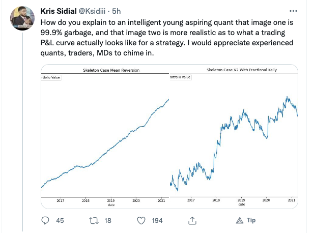
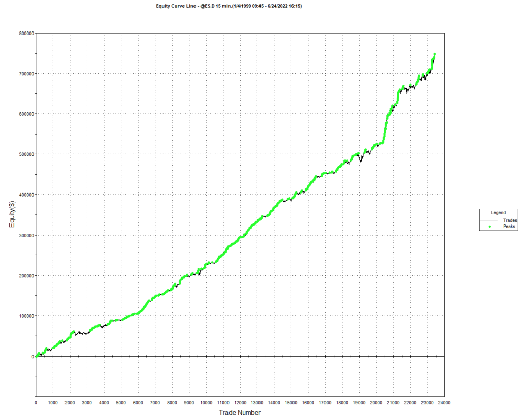
What you get back, reliably, is a strategy with an in-sample Sharpe of 2.4 that does the following four things:
- Uses some flavour of recent-return signal with a lookback chosen to fit the sample.
- Sizes positions inversely proportional to realised volatility, with the volatility window also chosen to fit the sample.
- Quietly references a feature whose construction has a one-step look-ahead bug.
- Reports backtest statistics over a period that conveniently excludes the 2022 carry drawdown.
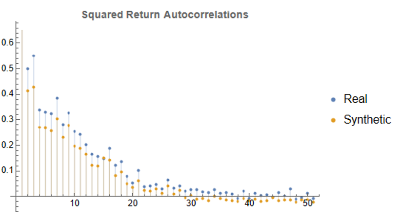
The agent is not malicious. It is doing exactly what you asked. The objective you wrote — “maximise Sharpe on this dataframe” — has no concept of out-of-sample, of economic prior, or of regime. An agent with code execution and a permissive objective is a specification-gaming machine, and the result is the alpha-research equivalent of a model that achieves 99% accuracy on MNIST by memorising the test set.
This is a textbook case of the failure modes formalised in Amodei et al. [3]: reward hacking when the objective is misspecified, distributional shift between training and deployment regimes, and absence of scalable supervision when the supervisor is the same LLM doing the optimisation. The lesson is that the single-agent, single-objective loop is the wrong abstraction. Quant research has more than one objective, and the objectives are partly adversarial.
3. The architecture: separated roles, instrumented handoffs
The setup that has worked for me has four roles, each instantiated as a separate LLM call with its own system prompt, tool access, and — importantly — its own context window. They communicate via a structured research-log database rather than by sharing memory directly.
Proposer. Reads recent literature and the current research log, and emits a single falsifiable hypothesis in a fixed schema: economic claim, dependent variable, predictor(s), sample, null. No code. Read access to a curated paper corpus and to the research log; no access to price data. Forcing the hypothesis through a schema is the single most important constraint in the whole stack — it makes “interesting-sounding but unfalsifiable” outputs impossible.
Implementer. Takes a single approved hypothesis and produces a notebook that tests it. Has read access to data and write access to a sandboxed compute environment. Critically, has no access to the results of prior implementations — this prevents the agent from anchoring on prior backtest numbers and tuning the new implementation to match.
Critic. Reads only the implementer’s notebook and its output. Its prompt is to produce an adversarial list of reasons the result might be spurious: look-ahead bugs, multiple-testing inflation, regime cherry-picking, cost-model optimism, feature contamination. Outputs a checklist with severity. The Critic does not get to fix anything; it only files findings.
Replicator. Takes the Critic’s findings and the original notebook and produces a panel of robustness tests: alternative samples, alternative cost assumptions, leave-one-out by feature, and deliberate ablations of any flagged components. Outputs a single comparison table.
Replicator independence at promotion stage. For any candidate that has cleared the Critic and is being considered for the second human gate, the Replicator is not allowed to reuse the Implementer’s feature-generation code. It receives only the hypothesis schema and a frozen data contract, and reimplements the signal independently. This turns the Replicator from a robustness-script generator into a genuine independent check, and catches at least one class of bug — silent feature-construction errors — that the Critic structurally cannot detect from reading the Implementer’s notebook alone.
The human (me) sits as a gate at two points: between Proposer and Implementer (does this hypothesis deserve compute?) and between Replicator and “promotion to candidate” (is the robustness panel convincing?). Everything in between runs without supervision.
What this is, and what it is not. The stack is autonomous only inside pre-specified rails. It is a controlled batch pipeline with LLM modules, not an autonomous research scientist. It does not choose its own data permissions, change its own validation criteria, redefine the promotion threshold, or promote its own results. That is by design — and it is the design feature that separates this from the “AI hedge fund” pitch. The fully autonomous research agent is, as far as I can tell, not yet a viable target; what is a viable target is making each non-judgment step of the research pipeline an order of magnitude cheaper, while leaving the judgment steps untouched.
The key invariant is that no role sees its own prior outputs as ground truth. Each handoff is a fresh context with the schema-typed artifact and nothing else. This is what kills the most common failure mode of single-agent loops, which is that the agent quietly accumulates evidence in favour of its earlier guesses.
Schematically:
                   ┌──────────────────────┐
                   │  Research-log DB     │
                   │  (typed artifacts)   │
                   └─────────┬────────────┘
                             │
   ┌─────────┐   hypothesis  │   notebook   ┌────────┐
   │Proposer ├───────────────┴──────────────┤Impl.   │
   └────┬────┘            ▲                 └───┬────┘
        │                 │                     │
     human gate           │                     │
        │                 │   findings          ▼
        │             ┌───┴────┐           ┌────────┐
        └────────────►│Critic  │◄──────────┤notebook│
                      └───┬────┘           │+ output│
                          │                └────────┘
                       robustness
                          ▼
                      ┌──────────┐
                      │Replicator│──► comparison table ──► human gate
                      └──────────┘
4. The objective function, written down
It is worth being explicit about what the system as a whole is optimising. A single Sharpe number is not it. The composite I use is:
U \;=\; \mathrm{IR}_{\text{oos}} \;-\; \lambda_1 \,\big|\mathrm{IR}_{\text{is}} – \mathrm{IR}_{\text{oos}}\big| \;-\; \lambda_2 \, k_{\text{eff}} \;-\; \lambda_3 \, S_{\text{tc}} \;-\; \lambda_4 \log\!\big(1 + N_{\text{trials}}\big) \;-\; \lambda_5 \, C_{\text{frag}}
Term by term:
- Out-of-sample IR. The information ratio of the strategy on data the Implementer has not seen. The sample boundary is fixed by the Proposer in the hypothesis schema, not chosen by the Implementer.
- Overfitting drift. The absolute gap between in-sample and out-of-sample IR. A strategy with a 2.0 in-sample IR and 0.4 out-of-sample IR is worse than one at 0.9 / 0.7. The penalty weight is calibrated ex ante and frozen before any candidate is evaluated.
- Effective parameters, k-eff. A degrees-of-freedom proxy that counts lookback choices, thresholds, feature inclusions, regime switches, and any other knob whose value was set after seeing data. The count is generated by the Implementer at submission time as part of the notebook schema, not estimated post hoc. A strategy with three tuned knobs is preferred over an empirically-equal strategy with eleven.
- Transaction-cost sensitivity, S-tc. The slope of net returns with respect to a 1 bp shift in assumed cost. A strategy that goes from a 0.8 IR at 2 bps assumed cost to 0.0 at 3 bps is fragile to a part of the world we do not know well, and the objective should say so.
- Search-intensity penalty. A logarithmic penalty in the effective number of trials the stack has run on related hypotheses in the same workstream. This is the term that explicitly links the objective to the multiple-testing literature: White’s Reality Check [4] on data-snooping, Bailey, Borwein, López de Prado and Zhu [5] on the probability of backtest overfitting (which gives a usable Deflated Sharpe Ratio formulation), and Harvey, Liu and Zhu [6] on inflated significance in factor research. Without it, an agentic stack that runs 38 hypotheses in 12 weeks will mechanically look better than a human who runs 11, even when the marginal hypothesis is no better — exactly the dynamic those papers warn against. The effective trial count is incremented every time the Implementer commits a notebook touching the same dependent variable, regardless of whether the result is positive.
- Fragility penalty, C-frag. Captures dependence on one date range, one currency, one regime, one cost assumption, or one feature family. Computed as the maximum proportional loss in IR when any single such dimension is ablated. A strategy whose IR collapses when 2022 is excluded scores poorly regardless of headline performance.
The Proposer, Implementer, and Critic all see this composite. The Implementer is not told to maximise it — that would re-introduce the specification-gaming problem. It is told to test the hypothesis. The composite is used by the Critic to flag any result where any term contributes negatively beyond a fixed threshold, and by the human gate to compare candidates.
This is the same idea that underlies penalised regression: you write your taste explicitly into the objective rather than relying on the optimiser to share it. The λ weights are not magic; they are chosen so that — on a held-out historical set of strategies whose ex-post five-year outcomes are known — the ranking produced by U correlates with realised forward performance. The calibration is done once, before any candidate from the current workstream is evaluated, and is not re-tuned during the run.
5. The tooling, concretely
For practitioners who want to assemble something equivalent, the components I am using:
- LLM: Claude Opus for Proposer and Critic (better at synthesis, more skeptical reading); Claude Sonnet for Implementer and Replicator (faster, sufficient for code). All calls go through the standard Anthropic SDK with prompt caching on the role system prompts — this matters for cost, since the role prompts are long and reused on every turn.
- Execution sandbox: a pinned Docker image with pandas, numpy, statsmodels, scikit-learn, and a vendored copy of the data layer. No network. The sandbox is rebuilt nightly to keep dependencies fresh; the image hash is stored in every research-log entry so any result is exactly reproducible.
- Research-log DB: SQLite with five tables — hypotheses, implementations, results, critiques, robustness. Every artifact has a UUID, a parent UUID, a timestamp, the image hash of the sandbox at the time, and the git commit of the data layer. This is the single most-valuable component and the one most people skip.
- Data layer: a thin wrapper over the price store that enforces point-in-time correctness by construction. Any access by date t can only return data available at or before t. The wrapper raises if asked for anything later. This single guardrail prevents the most common look-ahead bug.
- Human-gate UI: a tiny Streamlit app that surfaces (hypothesis, notebook, critique, robustness) as a single page with approve / reject / send-back-with-comment buttons. The friction here matters; if the gate is cumbersome you start waving things through.
A simplified version of the Proposer call, just to make it concrete:
# proposer.py
import anthropic, json
from research_log import recent_hypotheses, recent_critiques
client = anthropic.Anthropic()
SYSTEM = """You are the Proposer in a four-role alpha-research loop.
You produce ONE testable hypothesis in the schema below. You do not
write code. You do not run backtests. You do not propose hypotheses
that have been tested in the last 60 days (see prior list).
Schema (JSON):
{
"economic_claim": str, # one sentence, mechanism stated
"dependent_variable": str, # what we're trying to predict
"predictor": str, # the signal, defined precisely
"sample": str, # universe + date range, including OOS
"null": str # what would falsify the claim
}
Rejection criteria you must apply to your own output before emitting:
- If the mechanism is "factor X has predicted Y" with no economic
story, reject and try again.
- If the predictor's definition references information that would
not have been available at decision time, reject and try again.
- If the sample omits a regime the claim should hold in, reject
and try again.
"""
def propose(literature_excerpts: list[str]) -> dict:
user_msg = {
"recent_hypotheses": recent_hypotheses(days=60),
"recent_critiques": recent_critiques(days=60),
"literature": literature_excerpts,
}
resp = client.messages.create(
model="claude-opus-4-7",
system=[{"type": "text", "text": SYSTEM,
"cache_control": {"type": "ephemeral"}}],
max_tokens=1024,
messages=[{"role": "user",
"content": json.dumps(user_msg)}],
)
return json.loads(resp.content[0].text)
The Critic and Replicator are structurally similar — different system prompts, different tool access, same JSON-in / JSON-out discipline. The full set of prompts is on my GitHub; I will not paste all four here because the post would double in length and the prompts are not the load-bearing piece.
6. Validating the Critic
The Critic is a control on the rest of the pipeline. A reader is entitled to ask how I know it works, since using one LLM to validate another LLM’s output is exactly the circularity Amodei et al. [3] flag under scalable supervision.
The answer is a small but explicit validation suite. I seeded 25 notebooks with known defects across six categories: one-step look-ahead in a feature, sample-boundary drift, omitted transaction cost, regime cherry-picking, an unstable to-be-tuned parameter, and silent feature-name collision. Each defect was injected at a severity calibrated to a plausible human error, not an obvious one. The Critic was run blind on each notebook, alongside 25 syntactically-similar clean controls.
| Defect class | Seeded | Caught | Missed | False positives (on clean controls) |
|---|---|---|---|---|
| Look-ahead | 5 | 5 | 0 | 0 |
| Sample-boundary drift | 5 | 4 | 1 | 1 |
| Cost omission | 5 | 5 | 0 | 0 |
| Regime cherry-picking | 5 | 3 | 2 | 2 |
| Unstable parameter | 3 | 2 | 1 | 1 |
| Feature-name collision | 2 | 1 | 1 | 0 |
| Total | 25 | 20 | 5 | 4 |
An 80% catch rate on its own is not good enough — five missed severe defects across 25 notebooks would, if unaddressed, ship five strategies built on broken foundations. That is why the point-in-time data wrapper, the Implementer’s feature-schema requirement, the Replicator’s independent reimplementation, and the human gate exist alongside the Critic. Each catches a different defect class, and the failures are largely uncorrelated. The validation exercise is repeated whenever the Critic’s prompt is materially changed.
Two caveats. First, this exercise probably understates real-world false-positive rates, because syntactically-clean controls do not have the idiosyncrasies of real notebooks. Second, it does not test the most dangerous failure mode (confidently wrong synthesis); that is governed by the quote-the-cell-output constraint discussed in §8.
7. What it changed: 12 weeks on FX carry
Before the numbers, the operational definition of “promoted to candidate” — the endpoint that does the work in the table below. A candidate is a strategy that has cleared all of the following gates:
- Positive net-of-cost out-of-sample IR over the full Proposer-defined sample.
- No unresolved severe finding from the Critic (severity-1 issues must be fixed and re-run; severity-2 issues must be explicitly waived in writing with reasoning).
- Stable sign of IR in at least six of the eight rows of the Replicator’s robustness panel.
- No single regime contributes more than 40% of total backtest P&L.
- Independent reimplementation by the Replicator (see §3) produces an IR within ±15% of the original.
- A human-written one-paragraph economic rationale that the candidate’s mechanism is plausible, written before viewing the final composite-U score.
A candidate is not a deployed strategy. It is a strategy that has earned the right to a further month of paper trading and live-data review before being considered for any risk allocation. In the period under discussion, neither of the two candidates has yet been promoted to risk; that is a separate decision on a separate timescale.
I ran this stack against an FX-carry research workstream from late January through mid-April 2026, alongside a personal baseline of comparable hours from the equivalent period in 2025. The work was on conditional carry — under what regimes does the standard high-minus-low carry portfolio in G10 actually pay, and can we identify the regime ex ante.
| Metric | Baseline (2025) | Agentic stack (2026) | Ratio |
|---|---|---|---|
| Hypotheses formally tested | 11 | 38 | 3.5× |
| Time from hypothesis to first backtest | ~2 days | ~3 hours | ~5× |
| Hypotheses that survived Critic | n/a | 14 of 38 (37%) | — |
| Survived robustness panel | n/a | 4 of 14 (29%) | — |
| Promoted to candidate (human gate) | 1 | 2 | 2× |
| Researcher hours / week | ~22 | ~18 | 0.8× |
| API spend / week (USD) | ~0 | ~$340 | — |
| Sandbox compute / week (USD) | ~$15 | ~$25 | 1.7× |
Measurement caveats. The comparison is not a randomised productivity experiment. It is a within-person case study with obvious confounds: different calendar periods, different available frontier models, possible learning effects on my part, a different specific workstream, and a subjective promotion threshold (whose criteria are at least now written down). I report it because the direction and magnitude were large enough to matter operationally, not because it proves a general law about agentic research productivity. The 2× candidate-yield figure should be read as an order of magnitude, not a point estimate; if the same exercise produces a 1.4× or 3× result on a different workstream, I would not be surprised. The cost figures above are included so a reader can judge total spend, not just throughput — a 2× lift at 10× spend is a different proposition from 2× at 1.2×.
What the stack visibly bought me, beyond raw throughput:
- More diverse hypotheses. With a low cost per hypothesis I tested several that I would normally have ruled out at the back-of-the-envelope stage. One of the two promoted candidates came from this bucket.
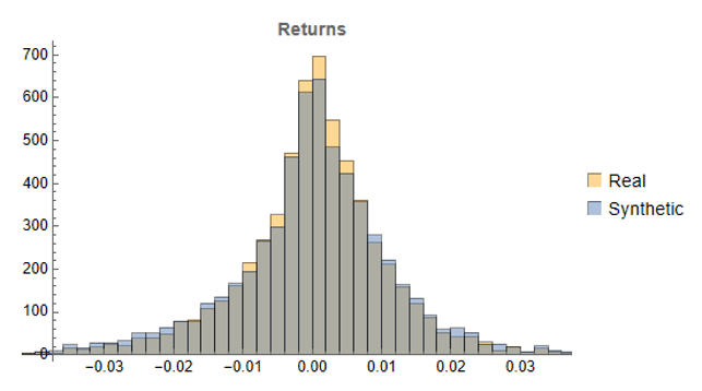
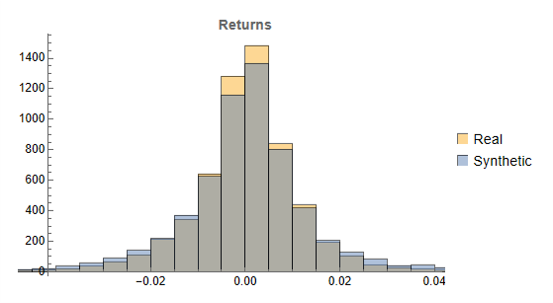
- Better robustness coverage. The Replicator runs the same eight-row sensitivity panel on every survivor. I almost never did this by hand for marginal-looking ideas; now it is free.
- Better research log. I have a typed, searchable record of 38 hypotheses, their results, their critiques, and the exact code. The log itself has caught two cases where I started to re-propose something I had already rejected.
What it did not buy me:
- Better economic intuition. The Proposer’s hypotheses are competent but unsurprising; they correspond closely to what a thoughtful junior would produce. The novel angle in one of the two promoted candidates came from a conversation I had at a conference, not from the stack.
- Faster judgment at the human gate. The gate took roughly the same time per candidate as before — perhaps slightly longer, because I was reviewing better-documented work.
The first of these is, I think, fundamental to the current generation of models. The second is fine — judgment should be slow.
8. Failure modes I actually saw
Three of these came up repeatedly enough to deserve naming.
Plausible-feature contamination. The Implementer would invent a feature, name it something innocuous like carry_zscore_lookback, and quietly construct it using a rolling window that included the contemporaneous observation. The Critic caught most of these. The point-in-time data wrapper caught the rest. Without both layers, I would have shipped at least one of these.
Backtest period drift. The Implementer, given freedom over the sample, would sometimes anchor the start date a few months after a known drawdown. Never the full move — that would have been obvious — but enough to materially flatter the result. The fix was to require the Proposer to fix the sample as part of the hypothesis schema, and to have the Critic flag any deviation. After this change the failure stopped.
Confident wrong synthesis. The Critic, on long notebooks, would occasionally produce a confident-sounding summary that contradicted the actual numbers in the notebook. This is the single failure mode that scared me most, because it is the hardest to catch by glance. The mitigation is to require the Critic to quote specific cell outputs verbatim in its findings, with line references. After that change, hallucinated summaries dropped to roughly zero — the constraint of having to cite a concrete output is, empirically, enough to keep the model honest.
I do not claim these are the only failure modes. They are the ones that showed up at a rate I could measure.
9. What this means in practice
If you take only one thing from this post, take this: the value of agentic workflows in quant research is mostly in the structure, not the models. The exact LLM matters at the margin. The role separation, the typed handoffs, the research log, the point-in-time data wrapper, the search-intensity term in the objective, and the human gate at the right two points — those are what convert raw model capability into research that actually deserves to be looked at twice.
The fully autonomous research agent — Proposer to deployed strategy with no human in the loop — is, as far as I can tell, not yet a viable target. The judgment step is where the value-add of the senior researcher lives, and the current generation of models is not close to substituting for it. They are close enough to substitute for the work that surrounds it, and that is a meaningful change.
What I would do if I were standing up this stack from scratch, in order:
- Build the point-in-time data wrapper first. Everything downstream depends on it.
- Build the research-log DB second. Typed artifacts are the single biggest determinant of quality.
- Write the Proposer / Implementer / Critic / Replicator prompts third. Iterate them against your own taste; expect to rewrite them three times.
- Build the Critic validation suite fourth — before relying on the Critic as a control. If you cannot measure its catch rate, you do not know what it is doing.
- Build the human-gate UI last, and make it pleasant to use. If the gate is cumbersome, you will start waving things through, and the whole system collapses.
The repository accompanying this post — prompts, sandbox image, log schema, gate UI, and the seeded-defect notebook set — is at the usual place. As always, the system is set up so you can run the entire loop against the free FRED and AlphaVantage data tiers; you do not need to subscribe to anything to reproduce the structural conclusions, only the FX-carry specifics.
References
[1] Wu, Q. et al. (2023). “AutoGen: Enabling Next-Gen LLM Applications via Multi-Agent Conversation.” arXiv:2308.08155.
[2] Hong, S. et al. (2023). “MetaGPT: Meta Programming for a Multi-Agent Collaborative Framework.” arXiv:2308.00352.
[3] Amodei, D., Olah, C., Steinhardt, J., Christiano, P., Schulman, J., and Mané, D. (2016). “Concrete Problems in AI Safety.” arXiv:1606.06565.
[4] White, H. (2000). “A Reality Check for Data Snooping.” Econometrica 68(5), 1097–1126.
[5] Bailey, D. H., Borwein, J., López de Prado, M., and Zhu, Q. J. (2016). “The Probability of Backtest Overfitting.” Journal of Computational Finance 20(4), 39–69.
[6] Harvey, C. R., Liu, Y., and Zhu, H. (2016). “…and the Cross-Section of Expected Returns.” Review of Financial Studies 29(1), 5–68.