
The Holdout That Made the Sharpe Bigger

First, a correction

The panel in my September post was supposed to have zero alpha. It didn’t quite. The market factor carried a drift of 0.0002 per day and the betas were drawn N(1, 0.3), so a book that tilted towards high-beta names had a true Sharpe of about +0.22 on a panel I described as containing nothing. The generator also clipped daily returns asymmetrically, at [−0.5, +1.0], which leaves a name whose shock breaches the floor with a small positive mean that a book ranking on volatility can load on.

I found this while building the generator for this study, and priced both defects rather than describing them. Every one of the 294 books that post reported on its zero-alpha panels — both reporting rules, all five arms — has been re-scored on the published panel and on a twin that differs only in having the drift removed. The twin is bit-identical otherwise: the drift constant consumes no random draws, so the two panels share every innovation. The recomputation reproduces all 294 published Sharpe ratios to machine precision (maximum absolute error 8.9 × 10⁻¹⁶).

The clip is the smaller of the two, and separable the same way. Across the twelve September panels it binds on 7 of 6,000,000 daily returns — a daily return above +50% is not a common event in a panel of 2%-volatility names — and a volatility-ranked book collects +0.003 of out-of-sample Sharpe from it (SE 0.002, largest on any single panel 0.02). The rest of this section is the drift.

September’s headline is an in-sample number, and in sample the drift is worth almost nothing: the median drift component of in-sample Sharpe across all 294 books is +0.006, and for the agent’s own books it is −0.007, against a published 2.24. Out of sample the median by arm runs +0.004 to +0.019, and no arm-and-rule cell exceeds +0.025, against +0.27 for a book constructed deliberately to load on beta — a different measurement from the +0.22 above, which is that book’s absolute Sharpe on the September panels rather than its drift component. Individual books move more — the largest is +0.49 and the smallest −0.22, and book beta loadings run from −0.21 to +0.25 — so the drift is not invisible at the level of a single run. The pre-registered threshold I had set for retracting a September conclusion, a median drift component above 0.101, does not fire.
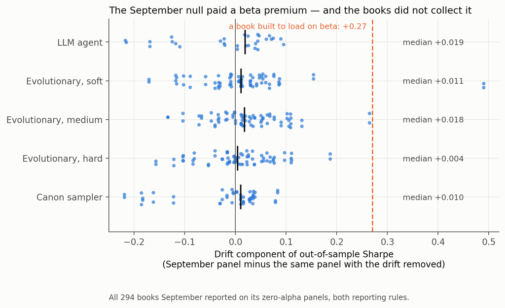
Every book September reported, on the published panel and on its drift-free twin

So September’s headline — that a research agent manufactures an in-sample Sharpe of 2.1 from nothing, and that 88% of it is explained by two integers in the log — stands. The generator does not. It has been replaced, the arithmetic is in the repository, and the correction is in this post rather than in a footnote, because a null you cannot verify is what this entire post is about.

Setup

The null. Factor-structured daily panels: 400 names, regime-switching volatility on the market and three latent factors, Student-t idiosyncratic shocks, lognormal dispersion in volatility. Zero drift, symmetric clipping, and — the part the September generator got wrong — separate random streams for structure (betas, loadings, volatilities, regime paths) and for innovations, so a fresh path can be drawn through the same world.

Verifying that a null is null is harder than writing one. The pre-registered acceptance test probed a constant-beta book and two oracle signals; it passed on two and, on the third, produced a +0.093 on the sixty study seeds that went away on a 120-seed replication. That episode is in the deviations file, and the acceptance file records the pre-registered failure rather than only the replication that passed. It also convinced me the test was too blunt, so there is a better one: 200 expressions drawn from the signal grammar before any panel existed, of which a median of 184 evaluate cleanly on a given panel, across 40 fresh null panels — 7,346 signal-panels, mean annualised Sharpe +0.017, 95% CI [−0.015, +0.048].

Two honest caveats on that. It is measured on the 1,000-day training window, not on the 2,000-day window the books are scored on. And on the exact sixty seeds this study ran, the residual tilt from the acceptance test is bounded at about +0.09 — larger than several of the out-of-sample numbers below. I flag them where they appear.

The pipeline being controlled. An evolutionary search over the same price-only grammar as the September post — returns, moving averages, rolling moments, range position, rolling beta and correlation, with cross-sectional and time-series normalisations. Twelve rounds of twenty-five expressions. The uncontrolled baseline reports the three highest in-sample Sharpes as an equal-weight book. Sixty seeds (9000–9059); 1,000 training days; 2,000 untouched days for scoring.

The two things worth measuring. Every control is placed on two axes.

How much manufactured Sharpe does it remove? Measured on panels with no alpha, and — this matters more than it sounds — measured on the number a user of that control would actually report. If a gate abstains, nothing is reported. If a control re-selects on a validation window, the researcher reports the validation-window number, not the training number they just threw away. If a control searches a shorter window, the researcher reports the shorter window’s Sharpe. Measuring every control on the original training window, which is what I did in the first pass of this study, flatters every re-selection control enormously and is the single largest correction here.

How much real alpha does it destroy? Measured on the same panels with a signal planted in them. Because each seed’s panels are drawn from identical innovations and differ only in the plant, the same book can be scored on both, which separates the exposure a noise-selected book has to the plant by construction from the gain that selecting on the planted panel actually adds. Only the second is “finding alpha”.

Two plants, and why. My first plant was calibrated to an in-sample Sharpe of about 1.0 — below the 1.77 the search manufactures from noise. A pipeline that ranks on in-sample Sharpe must then prefer the noise, so “the search fails to find real alpha” was a property of my calibration rather than a finding. There are now two, both calibrated on thirty seeds (8000–8029) rather than the three the first pass used: a weak plant and a strong one, with realised out-of-sample oracle Sharpes on the study seeds of 0.59 and 2.43.

The analysis plan, the predictions and the estimators were committed before the first search ran. Eighteen departures from them are logged, including several this study’s reviewers forced.

1. Selection manufactures the Sharpe. The search adds nothing.

Start with the uncontrolled pipeline on panels containing nothing:

Uncontrolled pipeline, 60 null panelsValue
Reported in-sample Sharpe1.77 (SE 0.04)
Realised out-of-sample Sharpe, 2,000 days+0.015 (SE 0.051)
One-way turnover, per day19.5%
Net of 5 bp per unit of turnover, at ≈2.5% book volatility−1.00

Familiar enough. Now the part I did not expect. Take 200 expressions drawn at random from the grammar before any panel is generated — no search, no feedback, no breeding — and keep the best three by in-sample Sharpe. On the same kind of null panel that book has an annualised in-sample Sharpe of 1.99 (SE 0.05, 40 panels).

Put the evolutionary search on exactly the same footing — its own logged candidates, the same 700-day window, the same complete-case filter, top three re-selected on that window — and it reports 1.95 (SE 0.05, 60 panels). The difference is 0.04, Welch t = 0.60.

Twelve rounds of adaptive search, three hundred evaluations, mutation and crossover, and the machinery adds nothing measurable to the manufactured number. Picking three things out of a hundred and eighty-odd does all of the work. (The two arms run on different seed sets and are not paired; the pools are matched at 182 against 184 candidates after filtering, with participation ratios of 13 and 15.)

Whatever your research process is — an agent, a grid, a graduate student with a notebook — the quantity that produces the fictitious Sharpe is the size of the set you chose from, and nothing clever has to have happened inside.

2. The holdout that made the number bigger

Here is the reported in-sample Sharpe on panels with no alpha, for each control, measured on the window that control actually reports:

ControlReported Sharpe, null panelsManufactured Sharpe removedAbstains
Internal gate (search 750 days, pick on 250)3.08−0.74—
Internal gate + leg cap of 12.45−0.38—
750-day search, no gate2.15−0.22—
Leg cap 121.78−0.01—
Uncontrolled baseline1.77——
Leg cap 11.650.07—
Budget 6 × 251.590.10—
Budget 12 × 121.560.12—
Budget 6 × 121.420.20—
Out-of-path gate (fresh innovations)1.360.23—
CSCV / PBO gate1.080.3925 of 60
Romano–Wolf stepdown0.410.7748 of 60
Deflated Sharpe hurdle0.001.0060 of 60

Read the last column before the middle one. For the three gates, the removal figure is driven by the abstention rate rather than by any reduction: those gates never make a fiction smaller. They make it rarer — and on the panels where Romano–Wolf does pass, the book it lets through reports 2.04, above the 1.77 it was meant to discipline; the PBO gate’s pass-conditional number is 1.85. That is why each gate’s removal figure sits below its abstention rate — 0.77 against 48 abstentions in 60, 0.39 against 25 — and it means that conditional on getting an answer out of them, you get a worse number than if you had not asked.

Now the top of the table. The train/validate split is the most widely practised control in quantitative research, and on a panel with no alpha it made the reported number 74% larger.

The mechanism is not subtle once you see it. On a panel with no alpha, every point of reported Sharpe is selection. The standard error of a Sharpe estimate scales as one over the square root of the sample, and for a fixed candidate pool the expected maximum scales with that standard error — so the ratio of two reported maxima should be the square root of the inverse ratio of their sample sizes. Those sample sizes are the days the Sharpe is actually computed over, after each book’s warm-up is dropped: 876 for the baseline, 591 for the 750-day search, and a clean 250 for the validation window, which needs no warm-up.

Predicted: √(876/591) = 1.2172 and √(876/250) = 1.872. Observed: 1.2175 and 1.742. The first is right to three decimal places. The gate falls a little short of its prediction because it selects from a pool bred on a different window, so its candidates are not the baseline’s candidates.

Look at the “750-day search, no gate” row, which is there precisely to separate the two effects. Running the same shorter search and reporting its own window’s top three already inflates the number by 22%. The gate adds a further 52 points of the baseline on top of that. Splitting the sample does not remove the selection: it relocates the selection to a shorter window, where selection is cheaper and its rewards are larger — and then hands you that number to report. This is the practical form of a result that is already well established in adaptive data analysis: a holdout reused for selection stops being a holdout [8].

The same logic hits the out-of-path gate, which I expected to be the best control in the study. It re-scores every candidate on a genuinely fresh path through the same world and keeps the best three. A top-three-of-two-hundred maximum over 1,000 fresh days is still worth 1.36. The gate does not remove the manufactured Sharpe. It moves it onto a new path and lets you report it there with a clear conscience.

If a control ends by selecting a maximum, the maximum is the problem, and the control has not addressed it.

One anticipation. A 750/250 split is not a straw split — 70/30 and 80/20 are the conventional choices, and the effect gets worse as the validation window shrinks, so a shop splitting 80/20 on four years is further along this curve than the one measured here.

3. The corrections are fine. You are pointing them at the wrong family.

Three of these controls are formal multiple-testing procedures with published guarantees: the deflated Sharpe ratio [1], the CSCV probability of backtest overfitting [2], and a Romano–Wolf stepdown at 5% familywise error [3], bootstrapped with a stationary block bootstrap [4]. Their realised size on null data is well known to be disappointing in practice. The question that seems not to get asked is whether that is the procedure’s fault.

So I measured each twice: once on the family of candidates the search produced, and once on a family of 200 expressions fixed before the data existed.
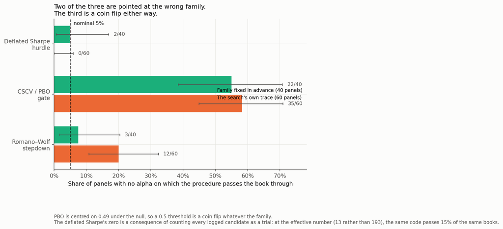
Realised size on a family fixed in advance against the search’s own trace

ProcedureFamily fixed in advance (40 panels)The search’s own trace (60 panels)
Deflated Sharpe hurdle2 of 40 (5%)0 of 60 at N = 193 logged; 9 of 60 (15%) at N effective = 13
CSCV / PBO gate22 of 40 (55%)35 of 60 (58%)
Romano–Wolf stepdown3 of 40 (8%)12 of 60 (20%)

On a family chosen before the data I can detect no inflation in either formal procedure. Forty panels is not enough to certify a 5% test — the Romano–Wolf interval runs from 1.6% to 20.4% — so read that column as the absence of the gross inflation the search family produces, not as a calibration certificate. What is unambiguous is the other side. Pointed at the family the search produced, Romano–Wolf rejects on 12 of 60 panels containing nothing: four times nominal, binomial p < 10⁻⁴. Forty panels against sixty is too little to make the 8%-versus-20% contrast itself significant — Fisher’s exact test on that comparison gives p = 0.15 — so the claim that carries is the one against nominal, not the one across columns. The size inflation on the search family is also not a bootstrap artefact: it holds at expected block lengths of 5, 21 and 63 days and at 500 and 2,000 replications, ranging from 18% to 20% across all four settings.

Why? Not because the bootstrap fails to see the generations that bred the survivors — restrict the family to the search’s round-zero population, random expressions no selection has touched, and rejections fall from 12 panels to 6 (paired exact p = 0.07). That points at adaptive breeding as one contributor rather than the whole story; on sixty panels it is a direction, not a decomposition. The rest is the plainer fact that the family was chosen by looking at the window the test then uses.

The deflated Sharpe ratio is a more uncomfortable case, because its answer is determined by a number you supply. It needs the number of trials; I gave it the count of distinct expressions the search logged, a mean of 193 across panels (range 103 to 258). Those are not independent trials — the participation ratio of their correlation matrix averages 13 (range 5 to 26). Feeding 193 independent trials into a formula that assumes independence pushes the expected-maximum benchmark above the book’s Sharpe on 40 of 60 panels, and leaves the z-statistic short of the 95th percentile on the other twenty — so the hurdle rejects everything. Feed it 13 and the same code, on the same books, passes 9 of 60 — three times nominal (p = 0.003), in the opposite direction. The control’s verdict is a function of a modelling choice nobody documents. To be clear, no published implementation asks for an effective trial count; this is an extension of the method, not a correction to it.

And then there is PBO, which I had been treating as a control and which is not one. CSCV’s logit statistic is symmetric about zero when the candidate strategies are exchangeable and null, so the probability of backtest overfitting is centred on 0.49 — by construction, not by accident. A threshold at 0.5 is therefore a coin flip on data containing nothing: it passes 55% of pre-specified null books and 58% of searched null books. It is not powerless — against the strong plant it passes 95% — but a gate whose false-pass rate is 58% is not a 5% test, whatever it does on real signal.

4. What the controls cost you

Removing fiction is half of a control’s job. The other half is not destroying the thing you are looking for, and you cannot measure that on a null panel.

Against the strong plant — realised out-of-sample oracle Sharpe 2.43, above what the search can manufacture — here is what each control finds of it, alongside what it removes:
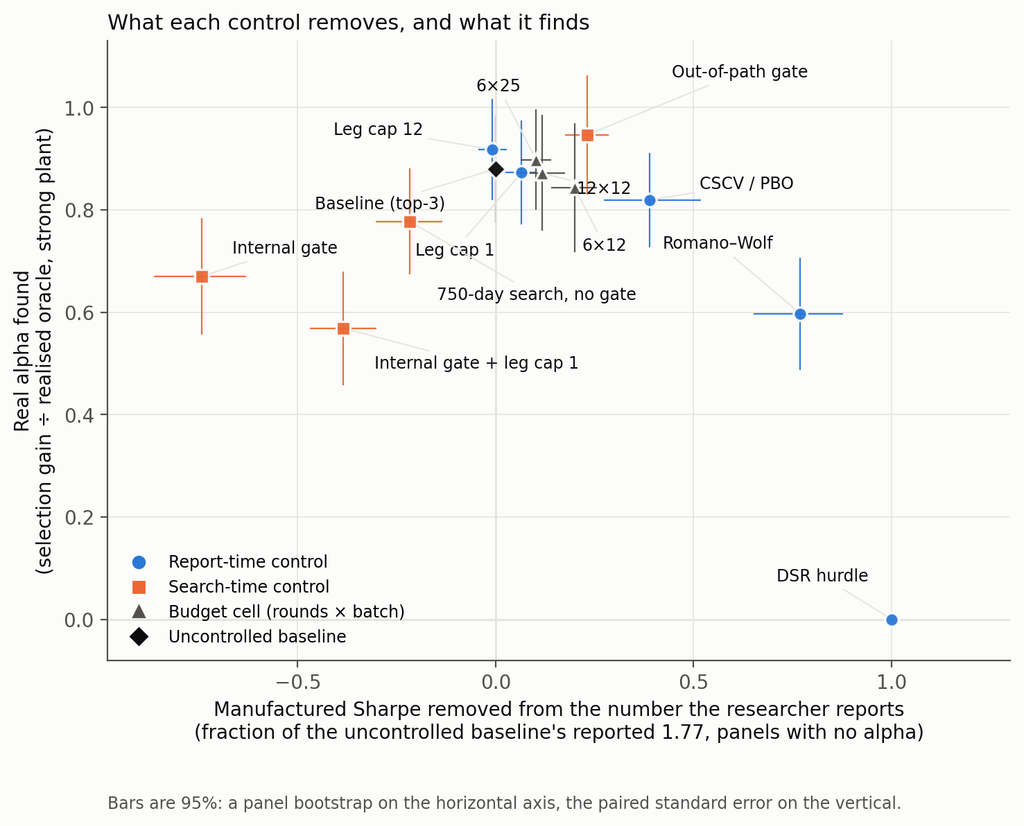
What each control removes and what it keeps

The right-hand column is the selection gain defined in the Setup — what selecting on the planted panel adds over what a null-selected book earns on it by construction. The raw ratio of book Sharpe to oracle is lower, because a book’s exposure to the plant is slightly negative on average: 0.81 for the baseline and 0.85 for the out-of-path gate.

ControlManufactured Sharpe removedReal alpha found (selection gain ÷ oracle)
Out-of-path gate0.230.95
Leg cap 12−0.010.92
Budget 6 × 250.100.90
Uncontrolled baseline—0.88
Leg cap 10.070.87
Budget 12 × 120.120.87
Budget 6 × 120.200.84
CSCV / PBO gate0.390.82
750-day search, no gate−0.220.78
Internal gate−0.740.67
Romano–Wolf stepdown0.770.60
Internal gate + leg cap 1−0.380.57
Deflated Sharpe hurdle1.000.00

The minimum difference detectable at 80% power between the baseline and any of the seven pre-registered controls in that column, after Holm across the whole 84-test scan, runs from 0.05 to 0.21 of the oracle. Differences smaller than that should not be read — including the gap between the out-of-path gate’s 0.95 and the uncontrolled baseline’s 0.88, which is nominally the largest in the table and is not separable at this sample size.

The deflated Sharpe hurdle rejects a genuine 2.4-Sharpe strategy on all sixty panels, and passes exactly one of the sixty carrying the weak plant. Its perfect score in the removal column and its zero in the retention column are the same fact stated twice. A control that abstains on everything is unfalsifiable on null data and useless on real data, and you cannot tell those two properties apart without running a planted arm.

Romano–Wolf is the most defensible trade in the table: it removes 77% of the fiction — by abstaining four times in five — and keeps 60% of a strong real signal. That is a real control with a real price, which is more than most of this column can claim.

The out-of-path gate keeps the most alpha while removing a real 23% of the fiction. It is the only control whose null-panel out-of-sample Sharpe is even marginally negative (−0.086, SE 0.045, 95% CI [−0.17, +0.00]) — a t of 1.9 in a scan across fourteen arms, and inside the residual-tilt bound I flagged in the Setup, so I would not lean on the sign.

Four controls dominate the internal gate on both axes after Holm adjustment: leg cap 1, leg cap 12, the out-of-path gate, and — awkwardly — the PBO gate I have just described as a coin flip. No other pair dominates. That a gate with no size control still dominates the internal gate says more about the internal gate than it does about PBO.

A fourteenth arm, the shorter search with a leg cap of 1, is in the repository and not in these tables: it reports 2.01 on null panels — a little less inflation than the window-matched arm’s 2.15 — and finds 0.78 of the plant, which is the window-matched arm’s figure to within noise.
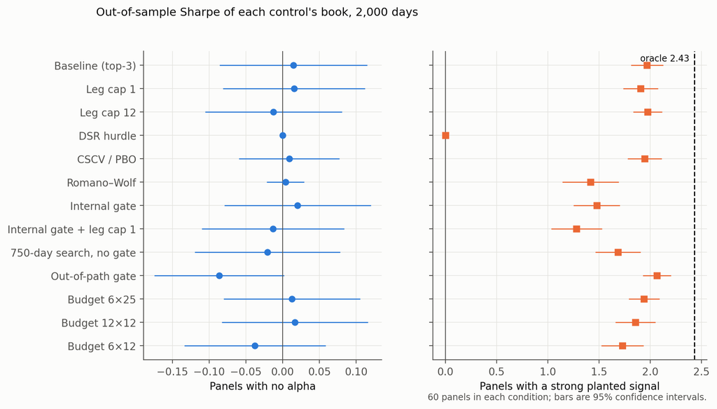
Out-of-sample Sharpe of each control’s book, with no alpha and with a strong plant

One more thing this table only shows because there is a strong plant in the study. Against the weak plant — oracle 0.59 — the uncontrolled pipeline’s selection gain is 11% of the oracle with a minimum detectable effect of 27%. That is not a finding, it is a non-detection, and the first pass of this study reported it as “the search captures 6% of the real signal”. The honest version is conditional and worth stating precisely: a search that ranks on in-sample Sharpe finds real alpha when the real alpha is larger than the alpha it can manufacture, and there is no evidence either way when it is smaller.

5. The agent behaves much like the machine

Eighteen fresh runs of the September research agent through a gated harness, six per condition, with the prompt frozen:

ConditionReported in-sampleRealised out-of-sampleOracleFound the plant
No alpha1.41−0.16 (SE 0.12)——
Weak plant1.52+0.24 (SE 0.17)0.503 of 6 exactly, 4 of 6 by family
Strong plant2.91+2.04 (SE 0.16)2.313 of 6 exactly, 6 of 6 by family

Manufactures on nothing, indistinguishable from noise against a weak signal, and its book earns 88% of the strong plant’s oracle out of sample against the mechanical pipeline’s 81% on the same raw basis. The arms ran on different panels and are not formally compared; qualitatively, whatever an LLM researcher is doing, it is not different enough from an evolutionary search to warrant a different control regime.

The arm is not blinded: the run id the agent types on every harness call carries the condition, K0, K1 or K2. Nothing in the logs refers to it, but it was in front of the agent, and six runs per condition is a small arm.

Two details worth having. The agents worked harder when there was more to find — 4.2 evaluation batches of a permitted 12 against the weak plant, 8.5 against the strong one — but they did not stop early on the null panel, where they used 5.7 batches and one run burned all twelve. That is responsiveness to signal strength, not an ability to notice there is nothing there.

And the twelve September agent traces, re-scored under the report-time controls on drift-free panels, behave as the mechanical arms do: the deflated Sharpe hurdle passes 0 of 12, PBO 5 of 12, Romano–Wolf 7 of 12. The exception is leg caps, which move an agent’s reported Sharpe by +0.02 on average at a cap of one and −0.02 at a cap of twelve — never by more than 0.29 on any single run, and in no consistent direction — because an agent’s legs live inside a single expression rather than in the count of expressions. Any control that counts expressions is close to blind to an agent.

6. One real path, for illustration

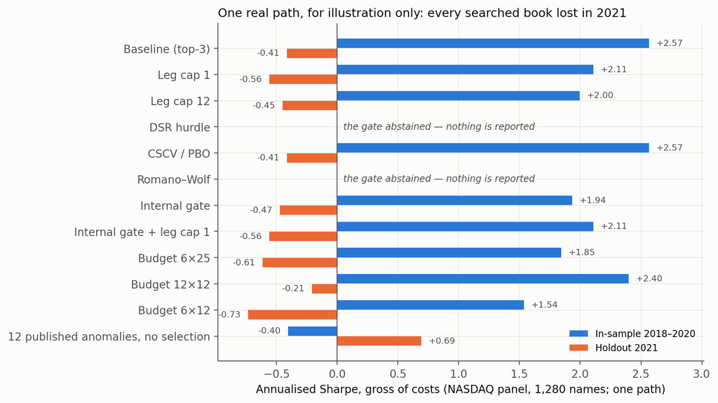
The same pipeline on a real panel — 1,280 NASDAQ names, search 2018–2020, holdout 2021 [5]. One path, a stale and survivorship-conditioned dataset, and a universe filter that looks at the whole sample. It evidences nothing; it is here because it makes the synthetic result legible.

BookIn-sample 2018–2020Holdout 2021Through May 2023
Baseline (top-3)+2.57−0.41−0.24
Leg cap 1+2.11−0.56−0.45
Leg cap 12+2.00−0.45−0.26
CSCV / PBO (passed)+2.57−0.41−0.24
Internal gate+1.94−0.47−0.26
Internal gate + leg cap 1+2.11−0.56−0.45
Budget 6 × 25+1.85−0.61−0.52
Budget 12 × 12+2.40−0.21−0.30
Budget 6 × 12+1.54−0.73−0.64
Deflated Sharpe hurdleabstained——
Romano–Wolfabstained——
Twelve published anomalies, no selection−0.40+0.69+0.69

Every searched book on the real panel, in sample and out

Every searched book turned negative. The unselected canon, which looked worst in sample, was the only thing that worked out of sample. Consistent with the synthetic result, and worth precisely as much as one path is worth.

One inconsistency to flag rather than let a reader find: the in-sample column here is the full 2018–2020 window for every book, including the internal gate, so it is not the reported-window number section 2 corrects to. On this arm the gate therefore appears to lower the in-sample figure when the synthetic result says it raises the number the gate’s user would report. The real panel’s dataset is fetched over the network and I could not re-score that row from the sandbox this study ran in; it is stated here rather than quietly left in the table.

The pre-registration scorecard

PredictionVerdict
P1 the out-of-path gate dominates the DSR hurdle on both axesRefuted, with each control winning one axis: the out-of-path gate removes 1.36 less of the reported Sharpe (CI [−1.45, −1.27]) and finds 2.07 more of the plant (CI [+1.92, +2.21])
P2 a leg cap of 1 removes ≥ 0.20 more than the smallest budget cellRefuted: −0.13, CI [−0.19, −0.07]
P3 the DSR hurdle’s size exceeds 25%Refuted: 0 of 60, conditional on N = logged candidates
P4a the internal gate costs ≥ 0.10 Sharpe on planted panelsConfirmed: −0.49, CI [−0.69, −0.29]
P4b the internal gate removes ≥ 0.50 of the manufactured SharpeRefuted, and in the opposite direction: −0.74

Things that did not work

The leg axis. Capping a book at one leg removes 0.13 less manufactured Sharpe than the smallest search budget does — the budget axis beat the leg axis, and leg caps are close to a no-op on this pipeline. Against an agent they are a complete no-op, for the reason in section 5. This is the one place where I expected a result from the literature to transfer and it didn’t: in-sample statistics do inflate with the number of combined signals [9], but not in a way a cap on the count can reach when the signals are themselves sums.

The pre-registered “oracle frontier” — thresholding candidates on their true out-of-sample Sharpe to trace the best attainable trade-off — is not reported at all. Estimating “true” out-of-sample Sharpe on the same window that scores the books is circular, and on null panels it obligingly produced a frontier that “retained” +0.60 of Sharpe that does not exist. The file is in the repository; the chart does not draw it.

And the first version of this study, which four reviewers took apart before publication. The largest correction was measuring each control on the number a researcher reports rather than the number they discard, which reversed the sign of the headline. The second was noticing that my planted signal had been calibrated to a level the search could beat by fabrication, which made one of my conclusions a property of the experiment rather than of the world. The third was catching three numbers quoted from the weak-plant arm where the text said otherwise. The fourth was showing that this post’s own draft compared the random family and the search on different windows, which inflated the gap in section 1 into a result it is not. All eighteen deviations are logged, and the first-pass tables sit in the repository beside the corrected ones.

What this does and does not show

It does show that on a verified-null panel an in-sample Sharpe of about 1.9 comes out of selecting three candidates from a couple of hundred, on the window the selection is made, and that twelve rounds of adaptive search add nothing measurable to that number.

It does show that a held-out validation window, used the way it is normally used, raises the reported Sharpe rather than lowering it, by roughly the factor the standard error of a Sharpe estimate predicts; and that a fresh-path re-test mostly relocates the manufactured Sharpe rather than removing it.

It does show that two of the three formal procedures show no detectable inflation on a family fixed in advance and are grossly mis-sized on a family the search selected; and that the third is centred on its own threshold under the null and therefore does not decide anything about size.

It does show that a pipeline, mechanical or agentic, recovers most of a planted signal strong enough to beat what it can manufacture — and that the deflated Sharpe hurdle, as conventionally parameterised, destroys all of it.

It does not show that any of these procedures is wrong. Each is implemented here against its published definition and is doing what it was designed to do on the input it is handed.

It does not show anything about faint alpha. Against a signal with a 0.59 oracle Sharpe this design cannot separate “finds nothing” from “finds a quarter of it”. That needs more panels or a longer scoring window.

It does not show a ranking of controls that transfers. The removal axis depends on the reporting convention, the retention axis on a plant that happens to be a single expression the grammar can write exactly — evaluated verbatim by the mechanical search on only 6 of the 60 strong-plant panels, so its findability is not an artefact of expressibility, but a plant the grammar cannot write at all would give a different answer. The leg-cap results depend on a grammar in which a leg is a separate expression, and every net-of-cost number on a book volatility of about 2.5%.

It does not show anything about real markets. One path on a stale dataset is an illustration.

So what do you do?

Report the number you selected on, and say which window it is. Most of the apparent power of every re-selection control in this study came from measuring it on a window the researcher had already discarded: the out-of-path gate’s removal falls from 0.99 to 0.23 when you do this properly, and the internal gate’s flips sign, from +0.47 to −0.74. If your validation split produces a Sharpe of 3.1 where your in-sample fit produced 1.8, the honest headline is 3.1, and the fact that it is larger should alarm you rather than reassure you.

Write down the family before you look. Not the trial count — the family. Every procedure in section 3 shows no inflation on a family fixed in advance and gross inflation on a family your search selected, and the difference between those is a decision you make before the data, not a correction you apply after it.

If you use the deflated Sharpe ratio, state how you counted trials, and report the effective number alongside the raw count. The gap between 193 and 13 on the same candidate set moved the pass rate from 0% to 15%. No published implementation asks for an effective count, so this is an extension rather than a fix — but a DSR quoted without saying how trials were counted is a number with a free parameter in it.

Stop using a PBO threshold of 0.5 as a gate. It is centred on 0.49 under the null. Use the distribution, or use something else.

Run a planted arm. This is the one that costs real effort and is worth it. A control that abstains on everything looks perfect on a null panel; you only find out what it costs when you give it something real to find. And calibrate the plant above what your own pipeline can fabricate, or you will measure your calibration rather than your control — which is exactly what the first version of this study did.

Code and data

The repository holds the pre-registered analysis plan committed before the first run, eighteen logged deviations from it, the corrected generator with its bitwise verification against the September panels, the calibration of both plants, the full study across 180 panels, the pre-specified-family placebo, the erratum arithmetic against all 294 previously published books, the agent harness with every run log and journal, the canary tests, and the analysis and figure code. Seeds: study panels 9000–9059, calibration 8000–8029, placebo panels 9500–9539, pre-specified family drawn from seed 20260921. Everything except the LLM calls reproduces from those seeds; the LLM calls are not re-runnable, which is why the logs are included in full. The repository is at github.com/jkinlay/research-controls; this article refers to commit c11241e.

Two requests of anyone re-running it. Fix your family before you look at the data, and keep the list. And run a planted arm alongside the null arm — half the results here are invisible without one.

References

[1] Bailey & López de Prado, The Deflated Sharpe Ratio: Correcting for Selection Bias, Backtest Overfitting and Non-Normality, Journal of Portfolio Management 40(5), 2014.

[2] Bailey, Borwein, López de Prado & Zhu, The Probability of Backtest Overfitting, Journal of Computational Finance 20(4), 2017; and Pseudo-Mathematics and Financial Charlatanism, Notices of the AMS 61(5), 2014, for the expected-maximum-Sharpe result.

[3] Romano & Wolf, Stepwise Multiple Testing as Formalized Data Snooping, Econometrica 73(4), 2005, 1237–1282. The stepdown implemented here is the one-sided studentised version at 5% familywise error.

[4] Politis & Romano, The Stationary Bootstrap, Journal of the American Statistical Association 89(428), 1994. Expected block length 21 days throughout. The section 3 size result is stable across that choice: 18% at a block length of 5, 20% at 21, 18% at 63, and 18% at 21 with 2,000 replications rather than 500.

[5] skfolio, load_nasdaq_dataset — daily adjusted closes, 1,455 NASDAQ constituents, 2018-01-02 to 2023-05-31, documented by its authors as a stale dataset not intended for investment or commercial use. Filtered here to 1,280 names with median price ≥ $5.

[6] Harvey & Liu, Backtesting, Journal of Portfolio Management 42(1), 2015 — the multiple-testing haircut the report-time controls in section 3 descend from.

[7] Harvey & Liu, False (and Missed) Discoveries in Financial Economics, Journal of Finance 75(5), 2020, on the two-sided cost of correction; section 4 is a direct measurement of the missed-discovery side. See also Chen, The Limits of p-Hacking: Some Thought Experiments, Journal of Finance 76(5), 2021, 2447–2480, for the argument that selection alone cannot account for the observed cross-section — the complement of the measurement in section 1.

[8] Dwork, Feldman, Hardt, Pitassi, Reingold & Roth, The reusable holdout: Preserving validity in adaptive data analysis, Science 349(6248), 2015. Section 2 is the practical, one-reuse form of the result that a holdout used for selection stops being a holdout.

[9] Novy-Marx, Backtesting Strategies Based on Multiple Signals, NBER Working Paper 21329, 2015, on the inflation of in-sample statistics with the number of combined signals — the leg axis that section 4 finds to be a no-op here.

Disclosure: I run systematic strategies. Nothing here is a recommendation, and no strategy discussed is one I trade. These are diagnostic quantities from a methodological experiment on synthetic data and one stale public dataset, not a track record.

A Sharpe of 2.1 From Nothing: The Second Number Your Agent Doesn’t Log

September 2026

I gave a research agent four years of prices with no predictable structure in them — none, by construction — and it came back with a long/short book, an in-sample Sharpe of 2.1, and a paragraph explaining the economics of an effect that does not exist.

That is the measurement in this post. The more useful result is the second one: 88% of that number is accounted for by two integers — how many backtests the agent ran, and how many of the winners it blended into the book it reported. Only one of those is in the log everybody proposes to collect.

This closes a sequence. In August, having built an agentic research pipeline in May and measured a 2× lift in hypotheses tested per week, I priced a risk I had not thought to price: independent research runs against the same model produce books correlated at 0.62, a crowding exposure that appears in nobody’s risk report. That post ended with a claim I stated and did not measure — that faster hypothesis generation makes overfitting worse rather than better. This is the measurement, and my pre-registered prediction about how it would come out was wrong.


The one property agentic research has that human research never had

Every multiple-testing correction in finance founders on the same rock: you cannot observe the denominator. Harvey, Liu and Zhu built their t-statistic hurdle on an estimate of how many factors had been tried across the profession, not how many were published [1]. Harvey’s 2017 AFA presidential address is largely an argument about unreported trials [2]. The Deflated Sharpe Ratio requires you to supply the number of trials, and its authors are candid that in practice you are guessing [3]. Each method asks the researcher a question the researcher cannot honestly answer: how many things did you try before this one?

An agentic pipeline is different in exactly one respect. It has to ask the harness for every backtest it runs. The trial count is not a memory or an act of professional honesty. It is a log file.

So I built a minimal research agent, gave it one tool, recorded everything, and checked what the log is worth. The short answer is that it is worth less than I expected, for a reason that turns out to be measurable and fixable.


Setup

The harness. One command: submit up to 25 expressions, receive their in-sample scores. At most 12 such calls. The agent never sees prices, dates, tickers, or the holdout — the panel is anonymised to integer asset IDs and an integer time index, and the holdout files were physically absent from the filesystem while the runs executed. Every submission is logged with a timestamp, alongside a one-line hypothesis per batch and a free-text journal. The run ends when the agent reports exactly three signals.

What a “book” is, and the two counts that matter. Every arm’s output is scored the same way: three signals, equal-weighted into one book. The pre-registered primary rule takes the three highest-scoring signals a run evaluated, not the three it chose to report — the gap between the two is small and is itself reported below. N is the number of trials in the log. k is the number of additive legs in the resulting book: three for a searcher whose signals are single expressions, more for one whose signals are themselves sums. Those two integers carry the whole argument.

The signal language. A small price-only grammar: returns, moving averages, rolling moments, range position, rolling beta and correlation to the equal-weight panel, plus cross-sectional and time-series normalisations and arithmetic. It is the grammar from the August post, which matters — it was fixed before this hypothesis existed. Each signal becomes a dollar-neutral, rank-weighted long/short book with a one-day implementation lag.

The comparison arms. Three mechanical arms plus a no-selection placebo. The two that search run at the agent’s interaction schedule — 12 rounds of 25 candidates, feedback once per round. Matching rounds rather than evaluations is deliberate: in adaptive data analysis the damage scales with how many times you look and act, not with the raw query count [4].

ArmWhat it is
AGENTThe LLM researcher above
OPTEvolutionary search over the same grammar, at three selection pressures (soft, medium, hard — how aggressively each generation is bred from the current leaders)
CANON-SAMPLERCanon-shaped expressions with jittered parameters, no feedback — prior direction without optimisation
CANON placeboTwelve published anomalies in the same grammar, no selection at all

The data. The primary setting is synthetic: factor-structured panels with regime-switching volatility and fat tails, and zero predictability by construction. Volatility is forecastable; returns are not. The true Sharpe of every signal is zero, so every point of in-sample Sharpe is selection, and I can generate independent panels at will. The second setting is the real NASDAQ panel from the August post — 1,280 names, 2018–2023, train through 2021, holdout 2022 to May 2023.

The analysis plan, estimators, inclusion rule and predictions were committed to git before the first agent run. The repo holds the commit history, every harness log with its batch notes and research journals, a manifest of all 227 attempted runs including the five abandoned and why, and a list of every deviation from the plan.


1. What a research agent does with data that contains nothing

Twelve independent zero-alpha panels, one agent run each, identical prompt to the real-panel runs.

Every run found something. Every run wrote a confident rationale. From the report of a run on a panel whose returns are serially unpredictable by construction:

“All three combine the two independently validated engines: long-horizon cross-sectional mean reversion (ma 120-250, plateau confirmed across ret, ma, minr and maxr formulations at horizons 60-250) and a weekly return echo (returns from days t-8 to t-5 predict positively, with a coherent oscillating lag profile).”

There is no echo. There is no reversal. There is nothing.

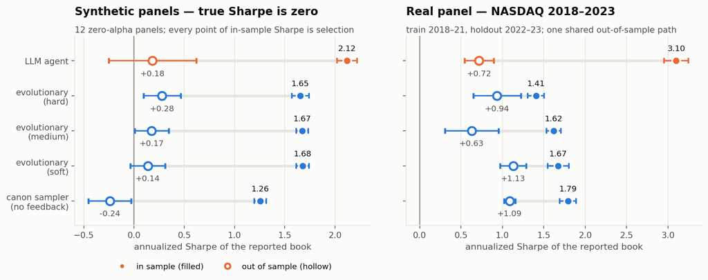
Zero-alpha panelsReported in-sample SharpeRealised out-of-sample Sharpe
LLM agent (12 runs)2.12 (SE 0.10)+0.18 (SE 0.44)
Evolutionary, soft (12 panels)1.68 (SE 0.07)+0.14 (SE 0.24)
Evolutionary, medium1.67 (SE 0.05)+0.17 (SE 0.22)
Evolutionary, hard1.65 (SE 0.11)+0.28 (SE 0.22)
Canon sampler, no feedback1.26 (SE 0.08)−0.24 (SE 0.29)

The reported book is the equal-weight composite of the three highest-scoring signals a run evaluated — the pre-registered primary rule, which is why it differs slightly from what the agent chose to report. True out-of-sample Sharpe is zero for every arm by construction, and every row is consistent with that. Standard errors are across panels.

A Sharpe ratio of 2.12, in-sample, on a book, over four years of daily data, from a panel with no signal in it.

A little over half of that is textbook. The expected maximum Sharpe of a single expression over the agent’s own median 146 logged trials is 1.15 (SE 0.03, across the twelve panels’ random-expression pools) — the expected-maximum-Sharpe effect [3], computed here as the exact order statistic over an empirical null pool drawn from the same grammar. That accounts for 54% of the 2.12. Note what the benchmark cannot do: those are single expressions, and it takes a single expression as the answer. Hold that thought — the missing 0.97 is the subject of section 3.

The agent’s own judgment is not the problem. It usually declines to report its top three by raw score, preferring what it calls “plateau” specifications; that restraint moves the number by 0.03 (2.08 chosen versus 2.12 argmax).

In-sample versus out-of-sample by search arm

2. It manufactures more than a machine built to overfit

Paired by panel, against the evolutionary optimiser at the identical interaction schedule, using only the twelve primary runs:

Contrast, in-sample Sharpe (12 paired panels)DifferenceSEt
Agent − evolutionary (soft)+0.440.11+3.9
Agent − evolutionary (medium)+0.450.11+4.1
Agent − evolutionary (hard)+0.460.09+5.2

On the real panel the gap is larger: 3.10 against 1.41–1.67.

That is the in-sample difference, and it is solid. The out-of-sample differences are not: those contrasts carry standard errors of 0.35 to 0.42, against a minimum detectable effect of about 1.0 Sharpe, and the pre-registered block bootstrap on the real panel returns a 95% interval of [−0.53, +1.99] for the agent’s realised Sharpe alone. Nothing in this study establishes that the agent’s books perform worse out of sample than a mechanical optimiser’s. What it establishes is that at a matched interaction budget, the agent converts noise into reported Sharpe more efficiently.

My pre-registered prediction was the opposite — that the model’s priors would act as a regulariser, keeping it in the published canon rather than in the noise, so it would overfit less. Wrong, at t ≈ 4.

3. Where the extra Sharpe comes from is not more searching

The mechanism is in the logs, and it is not model priors.

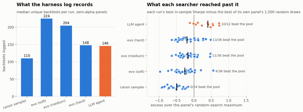
The agent logs a median of 146 unique backtests per zero-alpha run, against 148–225 for the evolutionary arms: level with the hardest setting, well below the softer ones. It is not searching harder — and note that the largest gap in the table above, +0.46, is against the arm that runs the same number of trials.

The difference is in what gets reported. Every run reports three signals, which are equal-weighted into one book. For the mechanical arms each of those three is a single expression, so the book has 3 legs. The agent’s three are themselves sums: a median of 4.2 legs each on zero-alpha panels, so its book carries about 12.5. That is the second integer, and no trial-count correction records it.

To isolate it I ran a controlled experiment on the zero-alpha panels with no agent involved: draw N random expressions, keep the top k by in-sample Sharpe, equal-weight them into a book, and record what the book reports.

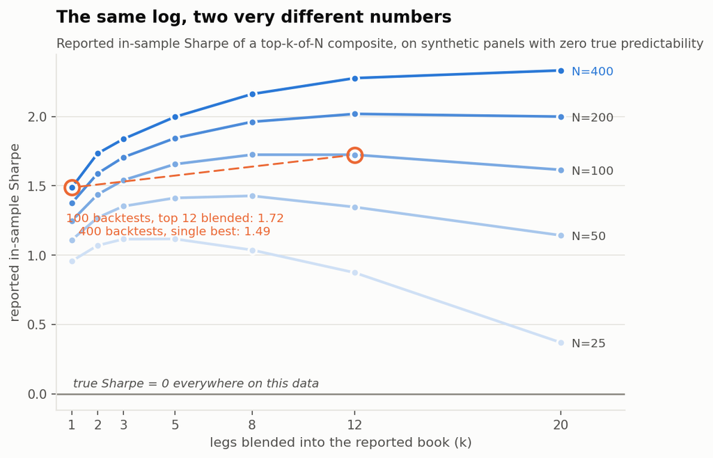
The selection-plus-aggregation surface

Moving between curves is the familiar overfitting-versus-trials axis. Moving right along a curve is the aggregation axis nobody logs. The two trade off against each other: a pipeline that logs 100 backtests and blends its top 12 reports 1.72, while one that logs 400 and reports a single best reports 1.49. No alpha in either case, and the first pipeline’s log looks four times cleaner.

The arithmetic is standard portfolio algebra pointed at noise. Selecting k signals on in-sample performance and averaging them keeps the selected mean and cuts the variance — but the legs are not independent, so the gain is √(k / (1 + (k−1)ρ̄)), not √k. Fitting that form column by column over the monotone region gives ρ̄ of 0.41–0.47 at the trial counts that matter here, a ceiling of about 1.5× however many legs you add. That is why the curves flatten. They turn down at small N for a different reason: once k is a large fraction of N you are averaging in candidates that were barely selected at all. Novy-Marx made the combination point for strategies built from multiple signals and derived corrected critical values for it [5]; what is new here is an agent that was never asked to combine anything doing it unprompted, and the interchangeability of the two axes at a fixed log.

The closure. Take each run’s own logged trial count and its own book leg count, look up what blind top-k-of-N selection produces at that point on the surface, and compare:

ArmMedian trialsLegs in bookBlind top-k-of-N predictsActually reportedResidual
LLM agent14612.51.862.12+0.26
Evolutionary, hard14831.681.65−0.03
Evolutionary, medium20531.731.67−0.05
Evolutionary, soft22531.771.68−0.09
Canon sampler11031.561.26−0.31

Two integers and no model price the evolutionary arms to within 0.09, and account for 88% of the agent’s number. The residual is +0.26 (t ≈ 2.1 once the surface’s own estimation error is propagated) — small next to the 1.86 that blind selection explains. And the leg axis alone carries most of the agent’s edge over the mechanical searchers: holding trials at the agent’s own 146 and moving the book from 3 legs to 12.5 adds +0.25, against a measured agent-minus-mechanical gap of +0.45.

So the agent beats the optimiser and is beaten by blind selection at its own operating point, and both facts have one cause. It blends; they do not.

That also settles what happened to the estimator I pre-registered. I had planned to report an effective trial count — the random draws from this grammar needed to match a run’s best score. It cannot be computed for most agent runs: 10 of 12 exceed the best their own panel’s 1,500-draw random pool reached, so no trial count reproduces them. That is partly a property of a finite pool and it is not agent-specific — 13 of 36 hard evolutionary runs also clear their pool — so nothing here rests on it. The direction is informative, though: a deeper random-expression pool (depth 6, mean complexity 5.9 against the shallow pool’s 3.6) lifts the 99th percentile from 0.95 to 1.24 and the maximum to 1.79 without closing the gap, because random expressions almost never build composites — mean legs 1.15.

Depth is not the axis. Blending is.

What the log records versus what random search reaches

4. The real panel

Six agent runs on the NASDAQ panel, trained through 2021, scored on 2022 to May 2023.

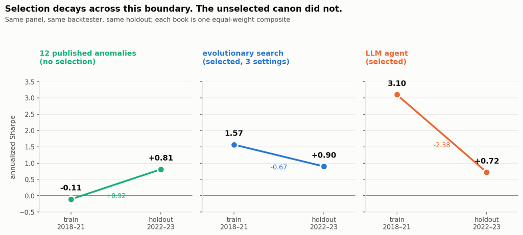
Real panelTrainHoldoutLegs in bookDaily turnover
LLM agent (6)3.10 (SE 0.15)+0.72 (SE 0.18)6.00.24
Canon sampler (5)1.79 (SE 0.10)+1.09 (SE 0.07)30.45
Evolutionary, soft (5)1.67 (SE 0.13)+1.13 (SE 0.16)30.43
Evolutionary, medium (5)1.62 (SE 0.09)+0.63 (SE 0.32)30.26
Evolutionary, hard (5)1.41 (SE 0.10)+0.94 (SE 0.29)30.49
12 published anomalies, no selection−0.11+0.81—0.14

The last row is the control that makes the rest interpretable, and it is scored exactly like every other row — one equal-weight composite, same backtester, same holdout — with no selection applied. It does not decay across this boundary. It improves, from −0.11 to +0.81. The 2022–23 environment was kinder to these exposures on this universe than the training window was.

So the regime component of the agent’s decay is not merely small; it is negative. The control licenses one claim and not a stronger one: the unselected canon did not decay here, so the regime cannot explain the agent’s 2.4-point gap. It does not follow that selection explains all of it — the canon composite is loaded the opposite way from a book selected to score 3.10 in the training window, and the pre-registered random-search leg that would have measured the selection component directly was not run.

Note what the ordering does not do. It is not monotone — the medium evolutionary arm has the lowest holdout Sharpe of any arm, below the agent’s — and every one of those holdout differences sits inside the block-bootstrap intervals. The real panel cannot adjudicate between these arms.

Turnover does not explain the gap either: the agent’s books turn over 24% of gross per day, at the low end of the arms rather than the high end.

The unselected canon did not decay across this boundary

5. What the number is worth, and what it is not

The obvious next move is to use the zero-alpha number as a correction: subtract what the pipeline manufactures from noise off the face value of what it reports on real data. Since true Sharpe on the synthetic panels is zero by construction, the manufactured component is the reported in-sample Sharpe itself — 2.12 for the agent. That gives 3.10 − 2.12 = 0.98 predicted against 0.72 realised, which looks like a hit.

It is not. Run the same arithmetic for every arm:

ArmZero-alpha manufactureReal facePredictedRealisedPredicted − realised
LLM agent2.123.100.980.72+0.26
Evolutionary, soft1.681.67−0.001.13−1.13
Evolutionary, medium1.671.62−0.050.63−0.68
Evolutionary, hard1.651.41−0.250.94−1.18
Canon sampler1.261.790.541.09−0.55

A negative last column means the haircut left too little on the table. Mean error −0.66. The correction under-predicts realised performance in four arms out of five, and the agent’s near-miss is the one that landed the other way. These are five books on one shared holdout path, not five independent draws, so this is one observation with five views of it rather than five tests. The reason is in the previous table: this holdout carried a tailwind of roughly +0.9 for canonical exposures, which a calibration built on noise cannot know about.

So the zero-alpha number measures how much in-sample Sharpe your pipeline manufactures from nothing. It is not a forecast of out-of-sample performance, because realised performance also contains whatever the regime does to your exposures, and that term is not small. What it is worth is the overstatement:

Selection overstatement — $100M book at 10% target volatility
Face in-sample Sharpe of the reported book3.1
Measured manufacturing capacity (zero-alpha calibration)2.1
Annual return overstatement≈ $21M
In basis points of notional≈ 2,100 bp

The amount by which the in-sample report overstates, measured on data containing no alpha. Gross of costs, rounded. Not a forecast and not strategy P&L: the row above shows the haircut does not predict realised returns. Absolute performance levels on a survivorship-conditioned panel are not defensible and no such claim is made.


Things that did not work

Two pre-registered predictions failed. The first, above: the prior did not act as a regulariser. The second concerned the planted-alpha panels, where I buried two effects of equal calibrated in-sample strength — one canon-shaped (short-horizon reversal), one deliberately anti-canon (a kurtosis effect the literature points away from) — expecting the agent to find the canon-shaped one better and the mechanical arms to show no such asymmetry. Both halves were wrong. At the higher plant strength the agent captured the anti-canon plant better (0.50 versus 0.41), and it was the evolutionary arm that showed the large asymmetry (0.87 versus −0.02) and delivered more of the real alpha out of sample (1.15 versus 0.50). The comparison is confounded — the plants were matched on in-sample strength, but their oracle holdout Sharpes came out at 0.46 and 1.30 — and the agent contributes four runs per cell.

A metric that dissolved against its null — for the second post running. Regressing the agent’s real-panel books on the twelve-anomaly basis gives a mean R² of 0.50: the agent is largely reproducing published anomalies. Run the same regression on random expressions from the same grammar and you get 0.72. Noise projects onto the canon basis better than the agent’s books do — so the metric ranks the agent as less canonical than random noise, which is not a statement about the agent at all. It measures the dimensionality of price-signal space. The lesson is cheap and general: any spanning statistic needs a null drawn from the same generator, or it is measuring the basis.

The look-ahead screen cannot fire. The holdout sits inside the model’s training corpus, so I pre-registered a one-sided screen against block-bootstrap continuations of the training panel — futures the model cannot have seen. Resampling training returns reproduces the structure the books were selected on, so the synthetic benchmark runs at 1.5–2.0 Sharpe for selected books and the statistic is negative by construction (Δ = −0.92; −1.64 under the demeaned variant). It found no evidence of pretraining leakage; it also could not have. The construction is in the repo.

The model changed underneath the experiment. Two-thirds of the way through, a rate limit forced a checkpoint switch. Four partly-completed runs were abandoned under the pre-registered inclusion rule and re-run on the same four panels; a fifth run was abandoned after I contaminated it with an operator timing probe. All five are in the manifest. The twelve primary zero-alpha runs are all on the first checkpoint. Three bridge runs on the second checkpoint over the same panels reported 2.74 against 2.09 for the first checkpoint on those panels. That gap is not identified, by this post’s own mechanism: the bridge runs used their full 300-trial budget against the primary runs’ ~145, and at fixed leg count the surface predicts about half of the 0.65 gap from trials alone. Three runs is an anecdote in any case; it is reported because it is the clearest available evidence that these numbers are a snapshot of specific checkpoints. Which checkpoint served each run was never recorded — it is reconstructed from run identifiers and timing, which is a defect in my instrumentation and is flagged in the repo.


What this does and does not show

It does not show that agent-generated books underperform mechanically-generated ones out of sample. Those contrasts are inside their standard errors and the design cannot resolve them.

It does not show that a zero-alpha haircut predicts realised performance. Section 5 shows it does not.

The limitations that matter, in order. This is a minimal single-loop researcher — one agent, one tool, ≤300 trials, no holdout gate, no research committee — one to two orders below a production pipeline, and everything a real stack adds either raises the trial count or is a control whose value this same instrumentation would demonstrate. It is a floor. One model family, and a checkpoint that changed mid-study; the cross-family experiment could not be run. The real panel is one shared out-of-sample path on a survivorship-conditioned universe inside the model’s training corpus, so every real-panel number here is descriptive and the inference lives in the synthetic arm. Twelve panels is a small cross-section and every interval is wide. And the mechanical arms are matched on rounds and grammar but not perfectly: the evolutionary arm is seeded and mutated at bounded expression depth while the agent writes free-form strings, so the agent searches a strictly larger subspace — which is consistent with the finding, since composite depth is exactly the axis that matters, but it means “same grammar” is doing less work than it sounds like.

Eleven deviations from the pre-registration — the censored trial-count estimator, the random-search decomposition leg that was not run, 60 continuations instead of 200, the warm-start evaluation basis, a prompt revised after the plan was committed, and the rest — are listed in DEVIATIONS.md.


So what do you do

Build the surface for your own stack. This is the differentiated move and it costs almost nothing. Construct a panel matched to your universe — same factor covariance, same volatility dynamics, same fat tails — with the conditional mean stripped out, and verify the construction by checking that an oracle signal earns zero. Then run your own pipeline against it, unmodified, and record what it reports at each (trials, legs) pair you actually operate at. That grid is your pipeline’s manufacturing capacity in the units you use, and you can look up any future result on it. For the pipeline here it was 2.1 Sharpe. The generator and the surface code are in the repo and the whole thing runs on a laptop.

Log two numbers, not one. The trial count is now an artifact rather than a memory, and a pipeline that cannot produce one is worse off than this toy. But on its own it prices nothing: a 12-leg book from 100 trials carries more selection than a single expression from 400, and only the first of those facts is in the log everyone proposes to keep. With both numbers you can look the answer up on your own surface. With one you cannot.

Then subtract, and stop there. The result tells you how much of the reported number is manufacturing. It does not tell you what the book will earn, because that also depends on what the regime does to your exposures — and section 5 shows that term is larger than the correction.

Every zero-alpha run in this study produced a good economic story — volatility term structure, lottery preference, reversal at horizons where reversal is documented — attached to nothing. The pipeline is a fine instrument. It is also, on data containing nothing, a machine for producing a Sharpe of 2.1 and a paragraph about why.


Code and data

Repo: jkinlay/agent-selection-surface

The repository contains the pre-registered analysis plan committed before the first run, a deviations list, the frozen prompt, the harness, the mechanical arms, the synthetic generator with its calibration constants, every run log with its batch notes and research journals, the manifest of all 227 attempted runs with dispositions and reasons, the backtester canary tests, and the analysis and figure code. Everything downstream of the LLM calls reproduces from seeds; the LLM calls are not re-runnable, which is why the logs are included in full.

Two requests of anyone re-running it. Run the zero-alpha arm first — it is what makes every subsequent number interpretable. And log the leg count, not just the trial count.


References

[1] Harvey, Liu & Zhu, …and the Cross-Section of Expected Returns, Review of Financial Studies 29(1), 2016.

[2] Harvey, Presidential Address: The Scientific Outlook in Financial Economics, Journal of Finance 72(4), 2017.

[3] Bailey & López de Prado, The Deflated Sharpe Ratio, Journal of Portfolio Management 40(5), 2014; Bailey, Borwein, López de Prado & Zhu, Pseudo-Mathematics and Financial Charlatanism, Notices of the AMS 61(5), 2014, for the expected-maximum-Sharpe result used in section 1.

[4] Dwork, Feldman, Hardt, Pitassi, Reingold & Roth, The reusable holdout: Preserving validity in adaptive data analysis, Science 349(6248), 2015 — guarantees degrade with the number of adaptive rounds, which is why every arm here is matched on rounds rather than evaluations.

[5] Novy-Marx, Backtesting Strategies Based on Multiple Signals, NBER Working Paper 21329, 2015 — in-sample test statistics inflate with the number of combined signals, with corrected critical values. The aggregation axis in section 3 is this effect, arrived at by an agent that was not asked to combine anything.

[6] skfolio, load_nasdaq_dataset — daily adjusted closes, 1,455 NASDAQ constituents, 2018-01-02 to 2023-05-31, documented by its authors as a stale dataset not intended for investment or commercial use. Filtered here to 1,280 names with median price ≥ $5; SHA-256 of the source file is in the analysis plan.

[7] Canonical anomalies in the placebo: Jegadeesh & Titman (1993) with the Carhart (1997) 12-1 construction; Jegadeesh (1990); Ang, Hodrick, Xing & Zhang (2006); George & Hwang (2004); Frazzini & Pedersen (2014); Boyer, Mitton & Vorkink (2010); Moskowitz, Ooi & Pedersen (2012); Novy-Marx (2012). The twelfth, a 60-minus-120-day momentum-acceleration variant, is a construction of my own.

Disclosure: I run systematic strategies. Nothing here is a recommendation, and no strategy discussed is one I trade. These are diagnostic quantities from a methodological experiment on a stale public dataset, not a track record.
Statistical Arbitrage with Synthetic Data

In my last post I mapped out how one could test the reliability of a single stock strategy (for the S&P 500 Index) using synthetic data generated by the new algorithm I developed.

Developing Trading Strategies with Synthetic Data

As this piece of research follows a similar path, I won’t repeat all those details here. The key point addressed in this post is that not only are we able to generate consistent open/high/low/close prices for individual stocks, we can do so in a way that preserves the correlations between related securities. In other words, the algorithm not only replicates the time series properties of individual stocks, but also the cross-sectional relationships between them. This has important applications for the development of portfolio strategies and portfolio risk management.

KO-PEP Pair

To illustrate this I will use synthetic daily data to develop a pairs trading strategy for the KO-PEP pair.

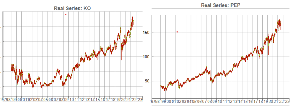
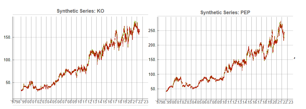
The two price series are highly correlated, which potentially makes them a suitable candidate for a pairs trading strategy.

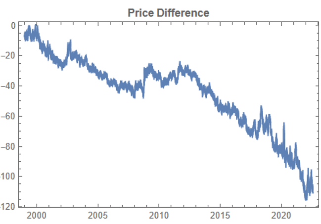
There are numerous ways to trade a pairs spread such as dollar neutral or beta neutral, but in this example I am simply going to look at trading the price difference. This is not a true market neutral approach, nor is the price difference reliably stationary. However, it will serve the purpose of illustrating the methodology.

Historical price differences between KO and PEP

Obviously it is crucial that the synthetic series we create behave in a way that replicates the relationship between the two stocks, so that we can use it for strategy development and testing. Ideally we would like to see high correlations between the synthetic and original price series as well as between the pairs of synthetic price data.

We begin by using the algorithm to generate 100 synthetic daily price series for KO and PEP and examine their properties.

Correlations

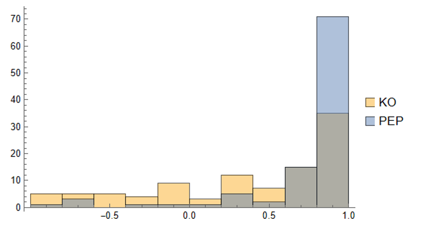
As we saw previously, the algorithm is able to generate synthetic data with correlations to the real price series ranging from below zero to close to 1.0:

Distribution of correlations between synthetic and real price series for KO and PEP

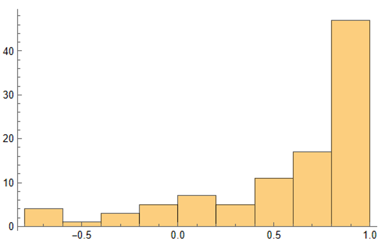
The crucial point, however, is that the algorithm has been designed to also preserve the cross-sectional correlation between the pairs of synthetic KO-PEP data, just as in the real data series:

Distribution of correlations between synthetic KO and PEP price series

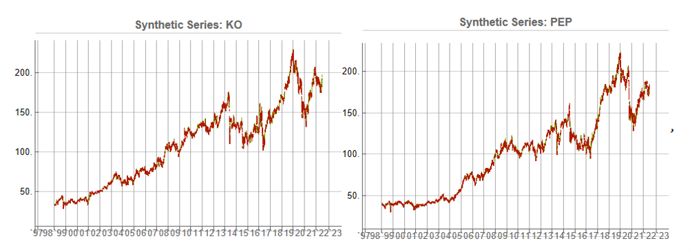
Some examples of highly correlated pairs of synthetic data are shown in the plots below:

In addition to correlation, we might also want to consider the price differences between the pairs of synthetic series, since the strategy will be trading that price difference, in the simple approach adopted here. We could, for example, select synthetic pairs for which the divergence in the price difference does not become too large, on the assumption that the series difference is stationary. While that approach might well be reasonable in other situations, here an assumption of stationarity would be perhaps closer to wishful thinking than reality. Instead we can use of selection of synthetic pairs with high levels of cross-correlation, as we all high levels of correlation with the real price data. We can also select for high correlation between the price differences for the real and synthetic price series.

Strategy Development & WFO Testing

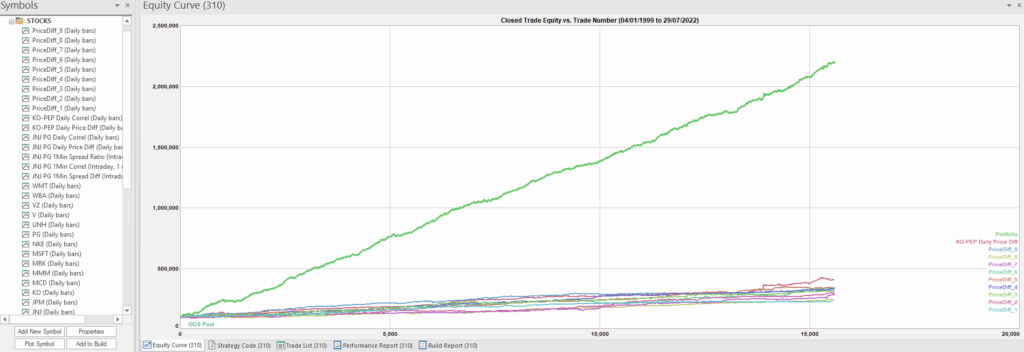
Once again we follow the procedure for strategy development outline in the previous post, except that, in addition to a selection of synthetic price difference series we also include 14-day correlations between the pairs. We use synthetic daily synthetic data from 1999 to 2012 to build the strategy and use the data from 2013 onwards for testing/validation. Eventually, after 50 generations we arrive at the result shown in the figure below:

As before, the equity curve for the individual synthetic pairs are shown towards the bottom of the chart, while the aggregate equity curve, which is a composition of the results for all none synthetic pairs is shown above in green. Clearly the results appear encouraging.

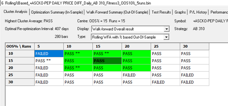
As a final step we apply the WFO analysis procedure described in the previous post to test the performance of the strategy on the real data series, using a variable number in-sample and out-of-sample periods of differing size. The results of the WFO cluster test are as follows:

The results are no so unequivocal as for the strategy developed for the S&P 500 index, but would nonethless be regarded as acceptable, since the strategy passes the great majority of the tests (in addition to the tests on synthetic pairs data).

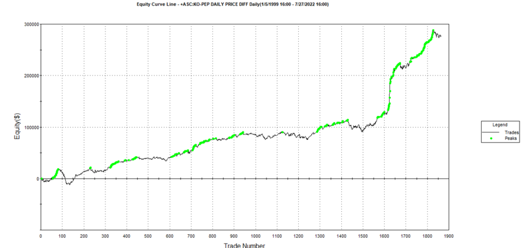
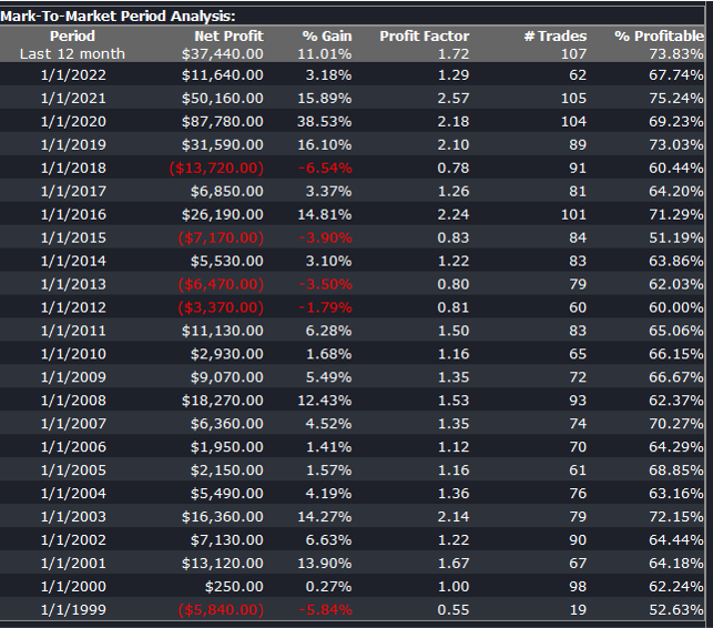
The final results appear as follows:

Conclusion

We have demonstrated how the algorithm can be used to generate synthetic price series the preserve not only the important time series properties, but also the cross-sectional properties between series for correlated securities. This important feature has applications in the development of statistical arbitrage strategies, portfolio construction methodology and in portfolio risk management.

Developing Trading Strategies With Synthetic Data

One of the main criticisms levelled at systematic trading over the last few years is that the over-use of historical market data has tended to produce curve-fitted strategies that perform poorly out of sample in a live trading environment. This is indeed a valid criticism – given enough attempts one is bound to arrive eventually at a strategy that performs well in backtest, even on a holdout data sample. But that by no means guarantees that the strategy will continue to perform well going forward.
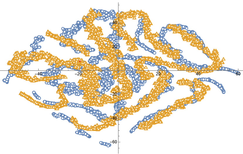
The solution to the problem has been clear for some time: what is required is a method of producing synthetic market data that can be used to build a strategy and test it under a wide variety of simulated market conditions. A strategy built in this way is more likely to survive the challenge of live trading than one that has been developed using only a single historical data path.

The problem, however, has been in implementation. Up until now all the attempts to produce credible synthetic price data have failed, for one reason or another, as I described in an earlier post:

I have been able to devise a completely new algorithm for generating artificial price series that meet all of the key requirements, as follows:

  • Computational simplicity & efficiency. Important if we are looking to mass-produce synthetic series for a large number of assets, for a variety of different applications. Some deep learning methods would struggle to meet this requirement, even supposing that transfer learning is possible.
  • The ability to produce price series that are internally consistent (i.e High > Low, etc) in every case .
  • Should be able to produce a range of synthetic series that vary widely in their correspondence to the original price series. In some case we want synthetic price series that are highly correlated to the original; in other cases we might want to test our investment portfolio or risk control systems under extreme conditions never before seen in the market.
  • The distribution of returns in the synthetic series should closely match the historical series, being non-Gaussian and with “fat-tails”.
  • The ability to incorporate long memory effects in the sequence of returns.
  • The ability to model GARCH effects in the returns process.

This means that we are now in a position to develop trading strategies without any direct reference to the underlying market data. Consequently we can then use all of the real market data for out-of-sample back-testing.

Developing a Trading Strategy for the S&P 500 Index Using Synthetic Market Data

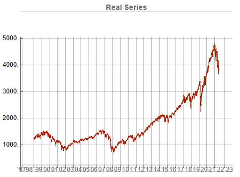
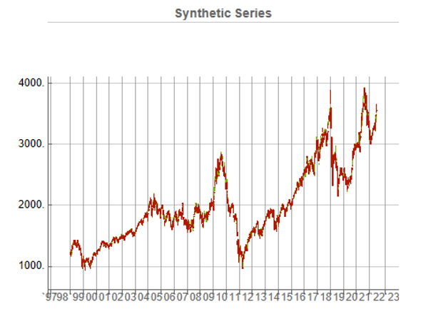
To illustrate the procedure I am going to use daily synthetic price data for the S&P 500 Index over the period from Jan 1999 to July 2022. Details of the the characteristics of the synthetic series are given in the post referred to above.

This image has an empty alt attribute; its file name is Fig3-12.png

Because we want to create a trading strategy that will perform under market conditions close to those currently prevailing, I will downsample the synthetic series to include only those that correlate quite closely, i.e. with a minimum correlation of 0.75, with the real price data.

Why do this? Surely if we want to make a strategy as robust as possible we should use all of the synthetic data series for model development?

The reason is that I believe that some of the more extreme adverse scenarios generated by the algorithm may occur quite rarely, perhaps once in every few decades. However, I am principally interested in a strategy that I can apply under current market conditions and I am prepared to take my chances that the worst-case scenarios are unlikely to come about any time soon. This is a major design decision, one that you may disagree with. Of course, one could make use of every available synthetic data series in the development of the trading model and by doing so it is likely that you would produce a model that is more robust. But the training could take longer and the performance during normal market conditions may not be as good.
Having generated the price series, the process I am going to follow is to use genetic programming to develop trading strategies that will be evaluated on all of the synthetic data series simultaneously. I will then use the performance of the aggregate portfolio, i.e. the outcome of all of the trades generated by the strategy when applied to all of the synthetic series, to assess the overall performance. In order to be considered, candidate strategies have to perform well under all of the different market scenarios, or at least the great majority of them. This ensures that the strategy is likely to prove more robust across different types of market conditions, rather than on just the single type of market scenario observed in the real historical series.
As usual in these cases I will reserve a portion (10%) of each data series for testing each strategy, and a further 10% sample for out-of-sample validation. This isn’t strictly necessary: since the real data series has not be used directly in the development of the trading system, we can later test the strategy on all of the historical data and regard this as an out-of-sample backtest.

To implement the procedure I am going to use Mike Bryant’s excellent Adaptrade Builder software.

This is an exemplar of outstanding software engineering and provides a broad range of features for generating trading strategies of every kind. One feature of Builder that is particularly useful in this context is its ability to construct strategies and test them on up to 20 data series concurrently. This enables us to develop a strategy using all of the synthetic data series simultaneously, showing the performance of each individual strategy as well for as the aggregate portfolio.

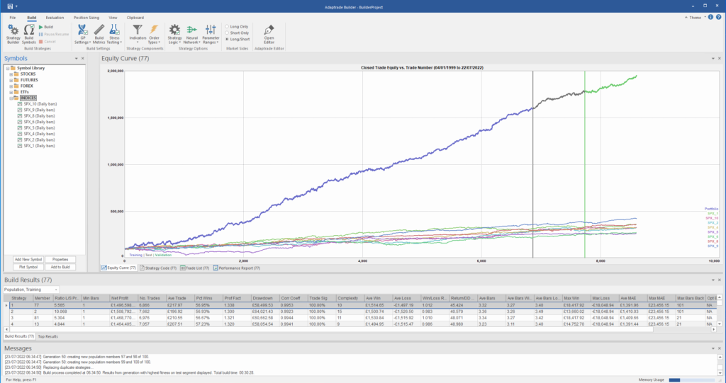
After evolving strategies for 50 generations we arrive at the following outcome:

The equity curve for the aggregate portfolio is shown in blue, while the equity curves for the strategy applied to individual synthetic data series are shown towards the bottom of the chart. Of course, the performance of the aggregate portfolio appears much superior to any of the individual strategies, because it is effectively the arithmetic sum of the individual equity curves. And just because the aggregate portfolio appears to perform well both in-sample and out-of-sample, that doesn’t imply that the strategy works equally well for every individual market scenario. In some scenarios it performs better than in others, as can be observed from the individual equity curves.

But, in any case, our objective here is not to create a stock portfolio strategy, but rather to trade a single asset – the S&P 500 Index. The role of the aggregate portfolio is simply to suggest that we may have found a strategy that is sufficiently robust to work well across a variety of market conditions, as represented by the various synthetic price series.

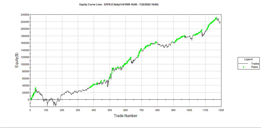
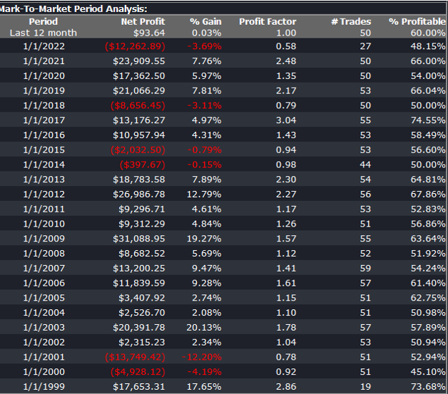
Builder generates code for the strategies it evolves in a number of different languages and in this case we take the EasyLanguage code for the fittest strategy #77 and apply it to a daily chart for the S&P 500 Index – i.e. the real data series – in Tradestation, with the following results:

The strategy appears to work well “out-of-the-box”, i,e, without any further refinement. So our quest for a robust strategy appears to have been quite successful, given that none of the 23-year span of real market data on which the strategy was tested was used in the development process.

We can take the process a little further, however, by “optimizing” the strategy. Traditionally this would mean finding the optimal set of parameters that produces the highest net profit on the test data. But this would be curve fitting in the worst possible sense, and is not at all what I am suggesting.

Instead we use a procedure known as Walk Forward Optimization (WFO), as described in this post:

The goal of WFO is not to curve-fit the best parameters, which would entirely defeat the object of using synthetic data. Instead, its purpose is to test the robustness of the strategy. We accomplish this by using a sequence of overlapping in-sample and out-of-sample periods to evaluate how well the strategy stands up, assuming the parameters are optimized on in-sample periods of varying size and start date and tested of similarly varying out-of-sample periods. A strategy that fails a cluster of such tests is unlikely to prove robust in live trading. A strategy that passes a test cluster at least demonstrates some capability to perform well in different market regimes.

To some extent we might regard such a test as unnecessary, given that the strategy has already been observed to perform well under several different market conditions, encapsulated in the different synthetic price series, in addition to the real historical price series. Nonetheless, we conduct a WFO cluster test to further evaluate the robustness of the strategy.

As the goal of the procedure is not to maximize the theoretical profitability of the strategy, but rather to evaluate its robustness, we select a criterion other than net profit as the factor to optimize. Specifically, we select the sum of the areas of the strategy drawdowns as the quantity to minimize (by maximizing the inverse of the sum of drawdown areas, which amounts to the same thing). This requires a little explanation.

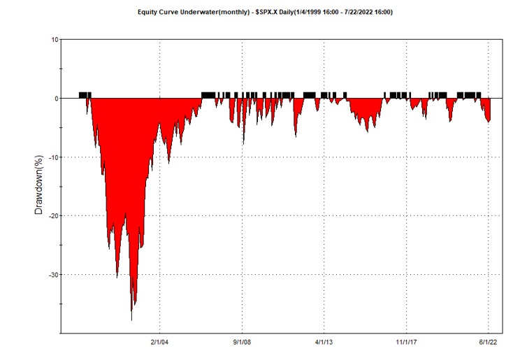
If we look at the strategy drawdown periods of the equity curve, we observe several periods (highlighted in red) in which the strategy was underwater:

The area of each drawdown represents the length and magnitude of the drawdown and our goal here is to minimize the sum of these areas, so that we reduce both the total duration and severity of strategy drawdowns.

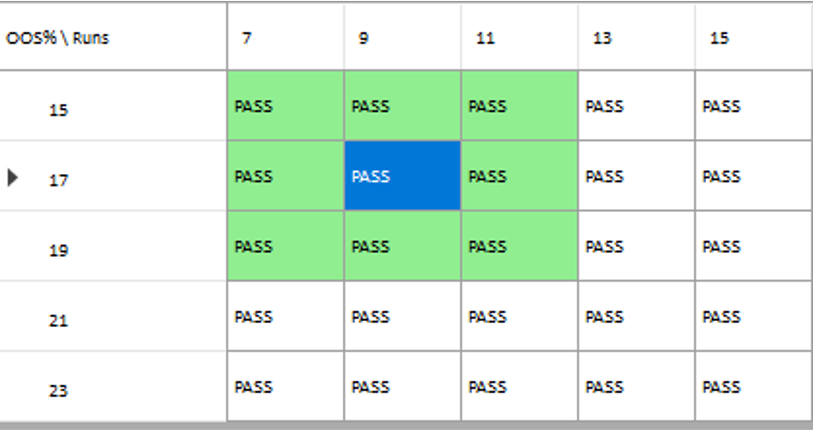
In each WFO test we use different % of OOS data and a different number of runs, assessing the performance of the strategy on a battery of different criteria:

x

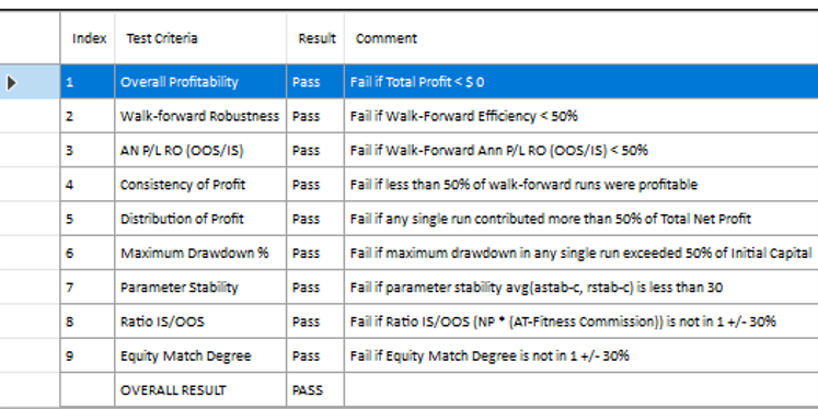
These criteria not only include overall profitability, but also factors such as parameter stability, profit consistency in each test, the ratio of in-sample to out-of-sample profits, etc. In other words, this WFO cluster analysis is not about profit maximization, but robustness evaluation, as assessed by these several different metrics. And in this case the strategy passes every test with flying colors:

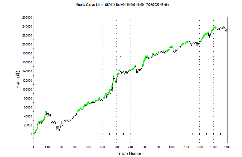
Other than validating the robustness of the strategy’s performance, the overall effect of the procedure is to slightly improve the equity curve by diminishing the magnitude and duration of the drawdown periods:

Conclusion

We have shown how, by using synthetic price series, we can build a robust trading strategy that performs well under a variety of different market conditions, including on previously “unseen” historical market data. Further analysis using cluster WFO tests strengthens the assessment of the strategy’s robustness.

A New Approach to Generating Synthetic Market Data

The Importance of Synthetic Market Data

The principal argument in favor of using synthetic data is that it addresses one of the major concerns about using real data series for modelling purposes: i.e. that models designed to fit the historical data produce test results that are unlikely to be replicated, going forward. Such models are not robust to changes that are likely to occur in any dynamical statistical process and will consequently perform poorly out of sample.

By using multiple synthetic data series following a wide range of different price paths, one can hope to build models – both for risk management and investment purposes – that can accommodate a variety of different market scenarios, making them more likely to perform robustly in a live market context.

Producing authentic synthetic data is a significant challenge, one that has eluded researchers for many years. Generating artificial returns series is a considerably simpler task, but even here there are difficulties. For many applications it is simply not sufficient to sample from the empirical distribution, because we want to produce a sequence of returns that closely mirrors the pattern of real returns sequences. In particular, there may be long memory effects (non-zero autocorrelations at long lags) or GARCH effects, in which dependency is introduced into the returns process via the square (or absolute value) of returns. These have the effect of inducing “shocks” to the returns process that persist for some time, causing autocorrelation in the associated volatility process in the process.

But producing a set of synthetic stock price data is even more of a challenge because not only do the above do the above requirements apply, but we also need to ensure that the open, high, low and closing prices are internally consistent, i.e. that on any given bar the High >= {Open, Low and Close) and that the Low <= {Open, Close}. These basic consistency checks have been overlooked in the research thus far.

Econometric Methods

One classical approach to the problem would be to create a Vector Autoregression Model, in which lagged values of the Open, High, Low and Close prices are used to predict the current values (see here for a detailed exposition of the VAR approach). A compelling argument in favor of such models is that, almost by definition, O/H/L/C prices are necessarily cointegrated.

While a VAR model potentially has the ability to model long memory and even GARCH effects, it is unable to produce stock prices that are guaranteed to be consistent, in the sense defined above. Indeed, a failure rate of 35% or higher for basic consistency checks is typical for such a model, making the usefulness of the synthetic prices series highly questionable.

Another approach favored by some researchers is to stitch together sub-samples of the real data series in a varying time-order. This is applicable only to return series and, in any case, can introduce spurious autocorrelations, or overlook important dependencies in the data series. Besides these defects, it is challenging to produce a synthetic series that looks substantially different from the original – both the real and synthetic series exhibit common peaks and troughs, even if they occur in different places in each series.

Deep Learning  Generative Adversarial Networks

In a previous post I looked in some detail at TimeGAN, one of the more recent methods for producing synthetic data series introduced in a paper in 2019 by Yoon, et al (link here).

TimeGAN, which applies deep learning  Generative Adversarial Networks to create synthetic data series, appears to work quite well for certain types of time series. But in my research I found it be inadequate for the purpose of producing synthetic stock data, for three reasons:

(i) The model produces synthetic data of fixed window lengths and stitching these together to form a single series can be problematic.

(ii) The prices fail a significant percentage of the basic consistency tests, regardless of the number of epochs used to train the model

(iii) The methodology introduces spurious correlations in the associated returns process that do not correspond to anything found in real stock return series and which get more pronounced as training continues.

Another GAN model, DoppleGANger, introduced by Lin, et. al. in 2020 (paper here) seeks to improve on TimeGAN and claims “up to 43% better fidelity than baseline models”, including TimeGAN. However, in my research I found that, while DoppleGANger trains much more quickly than TimeGAN, it produces a consistency test failure rate exceeding 30%, even after training for 500,000 epochs.

For both TimeGAN and DoppleGANger, the researchers have tended to benchmark performance using classical data science metrics such as TSNE plots rather than the more prosaic consistency checks that a market data specialist would be interested in, while the more advanced requirements such as long memory and GARCH effects are passed by without a mention.

The conclusion is that current methods fail to provide an adequate means of generating synthetic price series for financial assets that are consistent and sufficiently representative to be practically useful.

The Ideal Algorithm for Producing Synthetic Data Series

What are we looking for in the ideal algorithm for generating stock prices? The list would include:

(i) Computational simplicity & efficiency. Important if we are looking to mass-produce synthetic series for a large number of assets, for a variety of different applications. Some deep learning methods would struggle to meet this requirement, even supposing that transfer learning is possible.

(ii) The ability to produce price series that are internally consistent (i.e High > Low, etc) in every case .

(iii) Should be able to produce a range of synthetic series that vary widely in their correspondence to the original price series. In some case we want synthetic price series that are highly correlated to the original; in other cases we might want to test our investment portfolio or risk control systems under extreme conditions never before seen in the market.

(iv) The distribution of returns in the synthetic series should closely match the historical series, being non-Gaussian and with “fat-tails”.

(v) The ability to incorporate long memory effects in the sequence of returns.

(vi) The ability to model GARCH effects in the returns process.

After researching the problem over the course of many years, I have at last succeeded in developing an algorithm that meets these requirements. Before delving into the mechanics, let me begin by illustrating its application.

Application of the Ideal Algorithm

In this demonstration I am using daily O/H/L/C prices for the S&P 500 index for the period from Jan 1999 to July 2022, comprising four price series over 5,297 daily periods.

Synthetic Price Series

Generating ten synthetic series using the algorithm takes around 2 seconds with parallelization. I chose to generate series of the same length as the original, although I could just as easily have produced shorter, or longer sequences.

The first task is to confirm that the synthetic data are internally consistent, and indeed is guaranteed to be so because of the way the algorithm is designed. For example, here are the first few daily bars from the first synthetic series:

This means, of course, that we can immediately plot the synthetic series in a candlestick chart, just as we did with the real data series, above.

While the real and synthetic series are clearly different, the pattern of peaks and troughs somehow looks recognizably familiar. So, too, is the upward drift in the series, which is this case carries the synthetic S&P 500 Index to a high above 10,000 in 2022. Obviously this is a much more bullish scenario that we have seen in reality. But in fact this is just one example taken from the more “optimistic” end of the spectrum of possibilities. An illustration from the opposite end of the spectrum is shown in the chart below, in which the Index moves sideways over the entire 23 year span, with several very large drawdowns of -20% or more:

A more typical scenario might look something like our third chart, below. Here, too, we see several very large drawdowns, especially in the period from 2010-2011, but there is also a general upward drift in the process that enables the Index to reach levels comparable to those achieved by the real series:

Price Correlations

Reflecting these very different price path evolutions, we observe large variation in the correlations between the real and synthetic price series. For example:

As these tables indicate, the algorithm is capable of producing replica series that either mimic the original, real price series very closely, or which show completely different behavior, as in the second example.

Dimensionality Reduction

For completeness, as have previous researchers, we apply t-SNE dimensionality reduction and plot the two-factor weightings for both real (yellow) and synthetic data (blue). We observe that while there is considerable overlap in reduced dimensional space, it is not as pronounced as for the synthetic data produced by TimeGAN, for instance. However, as previously explained, we are less concerned by this than we are about the tests previously described, which in our view provide a more appropriate analysis benchmark, so far as market data is concerned. Furthermore, for the reasons previously given, we want synthetic market data that in some cases tracks well beyond the range seen in historical price series.

Returns Distributions

Moving on, we next consider the characteristics of the returns in the synthetic series in comparison to the real data series, where returns are measured as the differences in the Log-Close prices, in the usual way.

Histograms of the returns for the most “optimistic” and “pessimistic” scenarios charted previously are shown below:

In both cases the distribution of returns in the synthetic series closely matches that of the real returns process and are clearly non-Gaussian, with an over-weighting in the distribution tails. A more detailed look at the distribution characteristics for the first four synthetic series indicates that there is a very good match to the real returns process in each case (the results for other series are very similar):

We observe that the minimum and maximum returns of the synthetic series sometimes exceed those of the real series, which can be a useful characteristic for risk management applications. The median and mean of the real and synthetic series are broadly similar, sometimes higher, in other cases lower. Only for the standard deviation of returns do we observe a systematic pattern, in which returns volatility in the synthetic series is consistently higher than in the real series.

This feature, I would argue, is both appropriate and useful. Standard deviations should generally be higher, because there is indeed greater uncertainty about the prices and returns in artificially generated synthetic data, compared to the real series. Moreover, this characteristic is useful, because it will impose a greater stress-test burden on risk management systems compared to simply drawing from the distribution of real returns using Monte Carlo simulation. Put simply, there will be a greater number of more extreme tail events in scenarios using synthetic data, and this will cause risk control parameters to be set more conservatively than they otherwise might. This same characteristic – the greater variation in prices and returns – will also pose a tougher challenge for AI systems that attempt to create trading strategies using genetic programming, meaning that any such strategies are more likely to perform robustly in a live trading environment. I will be returning to this issue in a follow-up post.

Returns Process Characteristics

In the following plot we take a look at the autocorrelations in the returns process for a typical synthetic series. These compare closely with the autocorrelations in the real returns series up to 50 lags, which means that any long memory effects are likely to be conserved.

Finally, when we come to consider the autocorrelations in the square of the returns, we observe slowly decaying coefficients over long lags – evidence of so-called GARCH effects – for both real and synthetic series:

Summary

Overall, we observe that the algorithm is capable of generating consistent stock price series that correlate highly with the real price series. It is also capable of generating price series that have low, or even negative, correlation, a feature that may have important applications in the context of risk management. The distribution of returns in the synthetic series closely match those of the real returns process, and moreover retain important features such as long memory and GARCH effects.

Objections to the Use of Synthetic Data

Criticism of synthetic market data (including from myself) has hitherto focused on the inadequacy of such data in terms of representing important characteristics of real data series. Now that such technical issues have been addressed, I will try to anticipate some of the additional concerns that are likely to surface, going forward.

  1. The Synthetic Data is “Unrealistic”

What is meant here is that there is no plausible set of real, economic factors that would be likely to combine in a way to produce the pattern of prices shown in some of the synthetic data series. The idea that, as observed in one of the artificial scenarios above, the Fed would stand idly by while the market plunged by 50% to 60%, seems highly implausible. Equally unlikely is a scenario in which the market moves sideways for an extended period of a decade, or longer.

To a limited extent, I would agree with this. However, just because such scenarios are currently unlikely doesn’t mean they can never happen. For instance, take a look at the performance of the S&P 500 Index over the period from 1966 through 1979:

The market index barely made any progress throughout the entire 13-year period, which was characterized by a vicious bout of stagflation. Note, too, the precipitous drop in the index following the oil shock in 1973.

So to say that such scenarios – however implausible they may appear to be – can never happen is simply mistaken.

Finally, let’s not forget that, while the focus of this article is on the US market index, there are many economies, such as Mexico, Brazil or Argentina, for which such adverse developments are much more credible than they might currently be for the United States. We may wish to produce synthetic data for the markets in such economies for modelling purposes, in which case we will want to generate synthetic data capturing the full range of possible market outcomes, including some of the worst-case scenarios.

2. Extreme Scenarios Occur Too Frequently in Synthetic Data

Actually this is not the case – the generator tends to produce extreme scenarios with a frequency that is plausible, given the history and characteristics of the underlying, real price process. But there can be good reasons for wanting to control the frequency of such scenarios.

For instance, an investment manager may be looking to develop a “long-only” investment portfolio because, given his investment remit, that is the only type of investment strategy permitted. He would likely want to limit his focus to the more benign market outcomes for two reasons: (i) his investment thesis is that the market is likely to perform well, going forward (or else how does he pitch his strategy to investors?) and (ii) while he accepts that he may be wrong, it is not his job to hedge a possible market downturn – the responsibility for dealing with an adverse outcome falls to his risk manager, or to the investor.

Conversely, a risk manager is much more likely to be interested in adverse scenarios and, if anything, is likely to want to see such outcomes over-represented in a sample of synthetic data.

The point is, there is no “correct” answer: one has to decide which types of scenarios best suit the application one has in mind and sample the data accordingly. This can be done in a variety of ways such as setting a minimum required correlation between the synthetic and real price series, or designing a system of stratified sampling in which the desired outcomes are sampled according to a stipulated frequency distribution.

3. Synthetic Data Does Not Prevent Data Snooping and Curve Fitting

A critic might argue that, in fact, the real market data is “unseen” only in a theoretical sense, since its essential attributes have been baked into the synthetic series produced by the generator. This applies to an even greater extent if the synthetic series are sampled in some way, as described above.

I think this is a fair point. To take an extreme scenario, one could choose to select only synthetic series for which the correlation with the real data is 99.9%, or higher. Clearly this runs counter to the spirit of what one is trying to achieve with synthetic data and one might just as well use real data for modelling purposes. In practice, of course, even where a sampling methodology is applied, it is unlikely to be as crudely biased as in this example.

But, in any case, what is the alternative? The only option I can see is one in which a pure mathematical model is used to produce synthetic data, without any reference to the underlying real series. But, in that case, how would one assess the validity of the model assumptions, or how representative the synthetic series it produces might be?

There is no alternative but to have recourse to the real data at some point in the modelling process. In this procedure, however, the impact of snooping bias or curve fitting, even though it can never be totally extinguished, is very much diminished and it plays a less central role in model development.

Conclusion

It is now possible to produce synthetic data series that have all of the hallmark characteristics of real price data. This permits the analyst to investigate market models without direct recourse to the real price series, thereby minimizing data snooping and curve fitting bias. Models developed using synthetic data describing many different price path evolutions are more likely to prove robust across a wider range of plausible market scenarios in the real world.

In the next, follow-up post I will illustrate the application of synthetic data to the development of a robust investment strategy.