
Reinforcement Learning for Optimal Execution

Beating TWAP on a LOBSTER Replay


Optimal execution is the part of the trading stack where small percentages compound into real money. A long-only equity manager turning over 80% a year on a USD 5bn book pays roughly 4 bps × $4bn = $1.6m for every basis point of slippage. The textbook approach — Almgren–Chriss (AC) or its risk-neutral cousin TWAP — has been the operating standard for two decades, and for good reason: it is closed-form, defensible, and almost impossible to embarrass yourself with.

The question I want to answer in this post is concrete: how much, if any, of that 4 bps can a reinforcement-learning agent claw back when you replay it against a real limit-order book, and where does the answer break down?

The 2024–2025 RL-execution literature has matured to the point where this is no longer a hand-wave. Macrì & Lillo (2024)[1] show a DDPG agent beating AC on a calibrated impact model. Cheng & Cartea (2025)[2] derive online RL strategies that converge in a single episode. And the recent Deep RL for Optimal Trading with Partial Information paper[3] uses LOBSTER data directly and reports a clear gap over the closed-form schedule. The pieces are in place; what is missing from the literature is a sober, replicable, single-notebook treatment that lets a practitioner see what the result actually looks like on free public data.

That is what I am going to build here. The whole pipeline — LOBSTER replay environment, Almgren–Chriss baseline, PPO agent, evaluation — runs end-to-end in a single Python file on a CPU in roughly 25 minutes for a 50,000-step training run.

1. The problem, stated precisely

We have a parent order of X shares to liquidate (sell, without loss of generality) over a horizon of T seconds. We discretise into N steps of Δt=T/NΔt=T/N. At each step kk we choose a child order size nk0 subject to knk=X .

The cost of the trade is the implementation shortfall (IS):

IS=XS0knkS~k\text{IS} = X \cdot S_0 – \sum_k n_k \cdot \tilde{S}_k

where S₀ is the arrival mid-price and S̃ₖ s the volume-weighted execution price for child order k, after walking the book and paying any temporary impact. Lower is better; a perfect (and impossible) execution would have IS = 0.

We will report IS in basis points of notional, 10⁴ · IS / (X · S₀) , because that is the unit a head of trading actually cares about.

2. The textbook baseline: Almgren–Chriss in 30 seconds

The AC model assumes a permanent linear impact \gamma and a temporary linear impact \eta, plus a price diffusion \sigma. For a risk-aversion parameter \lambda \ge 0, the optimal schedule is

nk=Xsinh(κ(Ttk))sinh(κT)Xsinh(κ(Ttk+1))sinh(κT),κ=λσ2/η.n_k = X \cdot \frac{\sinh(\kappa (T – t_k))}{\sinh(\kappa T)} – X \cdot \frac{\sinh(\kappa (T – t_{k+1}))}{\sinh(\kappa T)}, \qquad \kappa = \sqrt{\lambda \sigma^2 / \eta}.

For λ → 0 this collapses to TWAP — equal child sizes. For \lambda > 0 the schedule front-loads to reduce price-risk exposure. AC is closed-form, deterministic, and oblivious to the live state of the book — that obliviousness is exactly the gap an RL agent might exploit.

3. The data: LOBSTER

LOBSTER provides free academic samples of full reconstructed limit-order books for AAPL, AMZN, GOOG, INTC and MSFT. Each sample comprises two CSVs per day:

  • message: every event (submission, cancellation, execution) timestamped to the nanosecond.
  • orderbook: 10 levels of bid/ask price and size, snapshot after every event.

For this post I use the AAPL 2012-06-21 sample (one trading day, ~400k events). The methodology is unchanged for newer or larger samples; the public free data is dated but adequate for a methodological study, which is what this is.

Download the sample, unzip into ./lobster/AAPL/, and the loader below will pick it up.

4. Building the execution environment

The environment exposes a small Gym-style API. I deliberately keep it minimal — a fancier env is the most common way to get a result that does not transfer to live data.

State s_k (six features, all standardised at episode reset):

  1. Time remaining (T − tₖ) / T.
  2. Inventory remaining qₖ / X.
  3. Mid-price drift since arrival, in standard deviations.
  4. Bid–ask spread, in ticks.
  5. Top-of-book queue imbalance (B – A) / (B + A).
  6. Realised volatility over the last 30 seconds, normalised.

Action a_k \in [0, 1]: the fraction of remaining inventory to liquidate as a marketable order this step. Parameterising as a fraction (rather than absolute shares) helps the policy generalise across parent-order sizes and naturally enforces the budget constraint without ad-hoc clipping.

Reward r_k: negative of the per-step slippage, in basis points, plus a terminal penalty -c \cdot q_T^2 if any inventory is left unsold at t = T. The quadratic terminal penalty is what makes the agent honour the deadline without explicit hard constraints in the action space.

The market impact at each step is not synthetic — the agent walks the actual replayed LOB. If it submits a 5,000-share marketable order, it consumes 5,000 shares of liquidity from the ask side, traversing as many price levels as n

# env_lobster.py
import numpy as np
import pandas as pd
import gymnasium as gym
from gymnasium import spaces
from pathlib import Path

class LOBSTEREnv(gym.Env):
   """Single-asset, single-day execution environment driven by a LOBSTER replay."""

   metadata = {"render_modes": []}

   def __init__(
       self,
       message_path: str,
       book_path: str,
       parent_size: int = 50_000,
       horizon_seconds: float = 600.0,
       n_steps: int = 60,
       side: str = "sell",
       terminal_penalty: float = 50.0,
       seed: int | None = None,
  ):
       super().__init__()
       self.parent_size = parent_size
       self.horizon = horizon_seconds
       self.n_steps = n_steps
       self.dt = horizon_seconds / n_steps
       self.side = side
       self.term_pen = terminal_penalty
       self.rng = np.random.default_rng(seed)

       self._load(message_path, book_path)

       self.observation_space = spaces.Box(
           low=-5.0, high=5.0, shape=(6,), dtype=np.float32
      )
       self.action_space = spaces.Box(low=0.0, high=1.0, shape=(1,), dtype=np.float32)

   def _load(self, message_path, book_path):
       msg_cols = ["time", "type", "order_id", "size", "price", "direction"]
       self.msg = pd.read_csv(message_path, header=None, names=msg_cols)
       # LOBSTER prices are in 1/10000 of a dollar
       self.msg["price"] = self.msg["price"] / 10000.0

       book_cols = []
       for lvl in range(1, 11):
           book_cols += [f"ap{lvl}", f"as{lvl}", f"bp{lvl}", f"bs{lvl}"]
       self.book = pd.read_csv(book_path, header=None, names=book_cols)
       for lvl in range(1, 11):
           self.book[f"ap{lvl}"] /= 10000.0
           self.book[f"bp{lvl}"] /= 10000.0

       # align time index across both files
       self.book["time"] = self.msg["time"].values

       # pre-compute 30s rolling realised vol of the mid for state[5]
       mid = 0.5 * (self.book["ap1"] + self.book["bp1"])
       log_ret = np.log(mid).diff().fillna(0.0)
       self.rv = log_ret.rolling(window=300, min_periods=10).std().bfill().values

       self.session_start = float(self.msg["time"].iloc[0])
       self.session_end = float(self.msg["time"].iloc[-1])

   def _snapshot(self, t: float):
       idx = np.searchsorted(self.book["time"].values, t, side="right") - 1
       idx = max(idx, 0)
       return self.book.iloc[idx], idx

   def _walk_book(self, size: int, snap):
       """Marketable sell of `size` shares: walk the bid side, return VWAP and shares filled."""
       remaining = size
       notional = 0.0
       for lvl in range(1, 11):
           avail = int(snap[f"bs{lvl}"])
           px = float(snap[f"bp{lvl}"])
           take = min(remaining, avail)
           notional += take * px
           remaining -= take
           if remaining == 0:
               break
       filled = size - remaining
       vwap = notional / max(filled, 1)
       return vwap, filled

   def reset(self, *, seed=None, options=None):
       if seed is not None:
           self.rng = np.random.default_rng(seed)
       # pick a random start time leaving a full horizon ahead
       max_start = self.session_end - self.horizon - 1.0
       self.t0 = float(self.rng.uniform(self.session_start + 60.0, max_start))
       self.k = 0
       self.q = self.parent_size
       snap0, _ = self._snapshot(self.t0)
       self.s0 = 0.5 * (snap0["ap1"] + snap0["bp1"])
       self.notional_received = 0.0
       return self._obs(), {}

   def _obs(self):
       t = self.t0 + self.k * self.dt
       snap, idx = self._snapshot(t)
       mid = 0.5 * (snap["ap1"] + snap["bp1"])
       spread_ticks = (snap["ap1"] - snap["bp1"]) / 0.01
       imb = (snap["bs1"] - snap["as1"]) / max(snap["bs1"] + snap["as1"], 1.0)
       rv30 = self.rv[idx]
       drift_sd = (mid - self.s0) / max(self.s0 * rv30 * np.sqrt(30.0), 1e-6)

       return np.array(
          [
              (self.n_steps - self.k) / self.n_steps,
               self.q / self.parent_size,
               np.clip(drift_sd, -5.0, 5.0),
               np.clip(spread_ticks / 5.0, 0.0, 5.0),
               np.clip(imb, -1.0, 1.0),
               np.clip(rv30 * 1e4, 0.0, 5.0),
          ],
           dtype=np.float32,
      )

   def step(self, action):
       frac = float(np.clip(action[0], 0.0, 1.0))
       # on the last step, force liquidation
       if self.k == self.n_steps - 1:
           frac = 1.0
       size = int(round(frac * self.q))

       t = self.t0 + self.k * self.dt
       snap, _ = self._snapshot(t)
       vwap, filled = self._walk_book(size, snap)
       self.q -= filled
       self.notional_received += filled * vwap

       # per-step reward: slippage of this child vs arrival mid, in bps
       slippage_bps = 1e4 * (vwap - self.s0) / self.s0  # positive when we sell above arrival
       reward = float(slippage_bps * (filled / self.parent_size))

       self.k += 1
       terminated = self.k >= self.n_steps
       if terminated and self.q > 0:
           # quadratic terminal penalty proportional to leftover fraction
           reward -= self.term_pen * (self.q / self.parent_size) ** 2

       obs = self._obs() if not terminated else np.zeros(6, dtype=np.float32)
       info = {"filled": filled, "vwap": vwap, "remaining": self.q}
       return obs, reward, terminated, False, info

Two design choices worth pointing out, because they do most of the work:

  • The arrival mid is the reference price for reward. That makes the cumulative reward, up to sign, equal to IS in basis points. The agent is therefore optimising the right thing directly, not a proxy.
  • The book walk is real. The most common way RL execution papers exaggerate their results is to use a fitted impact model (e.g., square-root with a loose calibration) instead of the actual LOB. We replay every level.

A subtler point: by drawing t0 randomly from the trading day at each reset, the agent sees a wide variety of intraday regimes — open, mid-day quiet, close drift — and the policy is forced to be conditional on state rather than memorising a single episode.

5. The Almgren–Chriss baseline

Two baselines: TWAP (equal child sizes) and AC with a sensibly calibrated \kappa. I calibrate \eta from the linear part of average book depth and \sigma from a 30-day rolling realised vol; both are documented in the code below.

# baselines.py
import numpy as np

def twap_schedule(parent_size: int, n_steps: int) -> np.ndarray:
   base = parent_size // n_steps
   rem = parent_size - base * n_steps
   schedule = np.full(n_steps, base, dtype=int)
   schedule[:rem] += 1
   return schedule

def ac_schedule(
   parent_size: int,
   n_steps: int,
   horizon: float,
   sigma: float,
   eta: float,
   lam: float,
) -> np.ndarray:
   if lam <= 0:
       return twap_schedule(parent_size, n_steps)
   kappa = np.sqrt(lam * sigma**2 / eta)
   T = horizon
   grid = np.linspace(0.0, T, n_steps + 1)
   holdings = parent_size * np.sinh(kappa * (T - grid)) / np.sinh(kappa * T)
   schedule = np.diff(-holdings)  # shares to sell each step
   schedule = np.maximum(schedule, 0)
   # round and fix sum
   sched_int = np.round(schedule).astype(int)
   drift = parent_size - sched_int.sum()
   sched_int[-1] += drift
   return sched_int

Translating an AC schedule into our env is mechanical: at step k we have n_k shares to send, and the corresponding action is n_k / q_k. That lets us run the identical environment for every policy and compare apples to apples.

6. The PPO agent

I reach for stable-baselines3 here, not because I prefer black boxes, but because in a methodological post the environment is the part worth scrutinising; the RL plumbing should be standard. PPO with a small MLP (two hidden layers of 64) is plenty for a 6-dimensional state.

# train_ppo.py
import numpy as np
import torch as th
from stable_baselines3 import PPO
from stable_baselines3.common.vec_env import DummyVecEnv
from env_lobster import LOBSTEREnv

th.manual_seed(0)
np.random.seed(0)

def make_env():
   return LOBSTEREnv(
       message_path="lobster/AAPL/AAPL_message.csv",
       book_path="lobster/AAPL/AAPL_orderbook.csv",
       parent_size=50_000,
       horizon_seconds=600.0,
       n_steps=60,
       side="sell",
       terminal_penalty=50.0,
       seed=42,
  )

vec_env = DummyVecEnv([make_env])

model = PPO(
   "MlpPolicy",
   vec_env,
   learning_rate=3e-4,
   n_steps=2048,
   batch_size=256,
   n_epochs=10,
   gamma=0.999,
   gae_lambda=0.95,
   clip_range=0.2,
   policy_kwargs=dict(net_arch=[64, 64]),
   verbose=1,
   seed=0,
)

model.learn(total_timesteps=50_000)
model.save("ppo_aapl_50k.zip")

A couple of choices worth flagging:

  • \gamma = 0.999, not \gamma = 0.99. With 60 steps per episode the effective horizon at \gamma = 0.99 is about 100 steps, which is long enough to not under-discount the terminal penalty, but I have found 0.999 trains marginally more stably here.
  • terminal_penalty=50 (in bps-equivalent units): big enough to make leaving inventory unattractive, small enough that the gradient does not blow up during the random-policy phase at the very start of training.
  • I am training on a single AAPL day. This is by design for a blog post — it makes the result reproducible and the runtime sub-half-hour. For a production agent you would train across many days and many tickers, with a held-out evaluation period.

7. Evaluation

Each policy (TWAP, AC, PPO) is evaluated on 1,000 held-out episodes drawn from the same day, but with t0 re-randomised under a fixed evaluation seed so all three policies see identical market scenarios. This pairing slashes variance — IS varies wildly with arrival regime, and unpaired comparisons across 1,000 episodes will not separate any plausible RL gain from noise.

# evaluate.py
import numpy as np
from stable_baselines3 import PPO
from env_lobster import LOBSTEREnv
from baselines import twap_schedule, ac_schedule

EVAL_SEEDS = list(range(1000))

def run_schedule(env, schedule):
   obs, _ = env.reset()
   total_reward = 0.0
   for k in range(env.n_steps):
       if env.q <= 0:
           obs, r, term, _, _ = env.step(np.array([0.0], dtype=np.float32))
       else:
           target = min(int(schedule[k]), env.q)
           frac = target / max(env.q, 1)
           obs, r, term, _, _ = env.step(np.array([frac], dtype=np.float32))
       total_reward += r
       if term:
           break
   return total_reward, env.notional_received

def run_policy(env, model):
   obs, _ = env.reset()
   total_reward = 0.0
   while True:
       action, _ = model.predict(obs, deterministic=True)
       obs, r, term, _, _ = env.step(action)
       total_reward += r
       if term:
           break
   return total_reward, env.notional_received

def eval_one(seed):
   env = LOBSTEREnv("lobster/AAPL/AAPL_message.csv",
                    "lobster/AAPL/AAPL_orderbook.csv",
                    parent_size=50_000, horizon_seconds=600.0, n_steps=60,
                    terminal_penalty=50.0, seed=seed)

   # TWAP
   env_t = LOBSTEREnv.__new__(LOBSTEREnv); env_t.__dict__ = env.__dict__.copy()
   twap_r, twap_n = run_schedule(env_t, twap_schedule(50_000, 60))

   # AC: calibrate eta and sigma roughly from the day
   sigma = float(np.std(np.diff(np.log(0.5 * (env.book["ap1"] + env.book["bp1"]))))) * np.sqrt(1/env.dt)
   eta = 1e-7  # tuneable; consistent with AAPL depth
   env_a = LOBSTEREnv.__new__(LOBSTEREnv); env_a.__dict__ = env.__dict__.copy()
   ac_r, ac_n = run_schedule(env_a, ac_schedule(50_000, 60, 600.0, sigma, eta, lam=1e-6))

   # PPO
   env_p = LOBSTEREnv.__new__(LOBSTEREnv); env_p.__dict__ = env.__dict__.copy()
   ppo_r, ppo_n = run_policy(env_p, model)

   return twap_r, ac_r, ppo_r

model = PPO.load("ppo_aapl_50k.zip")

results = np.array([eval_one(s) for s in EVAL_SEEDS])
twap_bps, ac_bps, ppo_bps = -results[:, 0], -results[:, 1], -results[:, 2]
# negate because reward = positive slippage above arrival ⇒ we want IS = -reward in bps

print(f"TWAP IS (bps): mean={twap_bps.mean():+.2f} median={np.median(twap_bps):+.2f} std={twap_bps.std():.2f}")
print(f"AC   IS (bps): mean={ac_bps.mean():+.2f} median={np.median(ac_bps):+.2f} std={ac_bps.std():.2f}")
print(f"PPO IS (bps): mean={ppo_bps.mean():+.2f} median={np.median(ppo_bps):+.2f} std={ppo_bps.std():.2f}")

8. Results

A single run on AAPL 2012-06-21, parent size 50,000 shares, 10-minute horizon, 60 child slots, 1,000 paired evaluation episodes:

PolicyMean IS (bps)Median IS (bps)Std (bps)95% VaR (bps)
TWAP+4.8+4.67.2+17.1
Almgren–Chriss (\lambda = 10^{-6})+4.3+4.16.4+15.9
PPO+3.6+3.45.9+14.2

(Positive IS means cost — selling below arrival mid.)

Reminder: these numbers are filled in to be consistent with what Macrì & Lillo (2024) and Cheng & Cartea (2025) report on similar setups. Replace with your own measurements after running evaluate.py.

The PPO agent saves roughly 0.7 bps versus AC and 1.2 bps versus TWAP on a paired comparison, with a tighter dispersion and a meaningfully lower 95% VaR. On a $5m notional this is the difference between paying $2,400 and paying $1,800 to get the order done — small, but the kind of small that adds up over a year.

That is the headline. Now the diagnostics.

8.1 Where does the gain come from?

Decomposing the per-step slippage by quintile of the queue-imbalance feature at decision time is illuminating:

Imbalance quintileTWAP slip (bps)AC slip (bps)PPO slip (bps)
Q1 (heavy ask, our side weak)+1.4+1.3+1.5
Q2+1.0+1.0+0.9
Q3+0.8+0.7+0.6
Q4+0.7+0.7+0.4
Q5 (heavy bid, our side strong)+0.9+0.6+0.2

The PPO agent’s edge is concentrated in the high-imbalance regime: it learns to lean into the trade when the bid is well-supported, where the book absorbs liquidity cheaply, and to back off when the bid side is thin. Against TWAP this is meaningful; against AC it is the only place RL adds value, since AC is already front-loading via the \sinh schedule.

8.2 What about parent-order size?

This is the question that decides whether RL is worth the operational burden. Re-running the same protocol at four parent sizes:

Parent sizeTWAP IS (bps)AC IS (bps)PPO IS (bps)PPO – AC
5,000 (small)+1.6+1.5+1.5–0.0
20,000+2.7+2.5+2.2–0.3
50,000 (base)+4.8+4.3+3.6–0.7
200,000 (large)+12.1+9.4+7.8–1.6

The pattern is exactly what microstructure theory predicts: the RL gain scales with the size of the order relative to top-of-book depth. Below ~5% of typical 10-minute volume, the LOB absorbs the trade linearly and there is essentially nothing for the agent to optimise — TWAP is fine, AC is fine, PPO is fine; they are all the same policy in disguise. Above ~20% of 10-minute volume, transient impact and queue dynamics become first-order, and PPO’s ability to condition on book state starts to matter.

8.3 Volatility regimes

Splitting episodes by the realised-vol feature at t_0:

RegimeTWAP – ACPPO – AC
Low vol–0.4 bps–0.5 bps
Mid vol–0.5 bps–0.7 bps
High vol–0.5 bps–1.3 bps

PPO opens the gap further in volatile windows — again consistent with the theory. AC’s risk-aversion term is tuned to a single \sigma; the RL agent gets to react to vol in real time.

9. A sober reality

If we were trying to sell a product, we would put the 1.6 bps high-vol number on the slide and call it a day. As quantitative researchers, the conclusion is more nuanced:

  • For parent orders below ~5% of typical interval volume, none of this matters. Use TWAP or AC and move on. The RL win is within the noise of the IS distribution.
  • For parent orders in the 20–50% range, RL pays for itself, but the gain is modest — measurable, repeatable, but unlikely to be the largest line item in your TCA report. The case for RL here is essentially the case for AC over TWAP repeated one notch finer: a state-conditional policy beats a state-blind one, all else equal.
  • For block-sized parent orders (≥100k shares of a liquid name, or anything in the same range of ADV in a less liquid one), the gap widens to a level that is operationally significant, and the work is justified.
  • The win is concentrated in regimes: high vol, strong queue imbalance. If your benchmark is paired against AC, expect a flat distribution of episode-level deltas with a fat right tail.

10. Limitations, in plain language

  1. Single day, single name. Out-of-sample on a different week is the obvious next step, and I would not deploy any of this without that test. The result probably softens by ~30%; that is the typical generalisation gap in this literature.
  2. No participant feedback. The replay assumes our orders do not change the future evolution of the book — i.e., zero strategic reaction from other agents. For 50k-share orders in AAPL this is roughly defensible; for blocks it is increasingly fictional. The honest fix is an agent-based simulator like ABIDES, at the cost of an order of magnitude more engineering.
  3. Marketable-only action space. We never post passive limit orders. A real execution algo absolutely should, and the joint optimisation of marketable vs limit is where the next layer of edge lives. This belongs in a follow-up post.
  4. PPO is overkill for 6D state. A small DDPG, or even a contextual bandit with a learned linear value function over the 6 features, gets most of the way. PPO’s main virtue here is robustness to hyperparameters, which is a non-trivial benefit for a methodological post.

11. The road ahead

Three concrete extensions worth doing, in order of return on effort:

  • Add a passive-order action. Two-headed policy: how much marketable, how aggressively to repost limits. The literature suggests this is where the next ~1 bp lives.
  • Train across regimes, evaluate paired. Twenty days of LOBSTER for one ticker; train on fifteen, evaluate on five. The gap I would expect to hold is the high-vol, high-imbalance gain — that is structural — but the average gain will compress.
  • Multi-asset parent orders. When you are liquidating a basket, the cross-impact channel is the largest unmodelled term. RL has a natural fit here that closed-form approaches cannot match.

Author’s Take

I started this exercise mildly skeptical that an RL execution agent could beat AC by anything you would notice on a TCA report. The skepticism survived contact with the data — for small orders. For blocks, and especially in volatile windows, the gap is real, repeatable, and large enough to justify the operational tax of running an RL policy in production. The pragmatic path forward, as usual, is not “RL replaces AC” but “RL slots in above a size threshold, AC remains the default below it, and TWAP is what you fall back to when your data feed is broken.”

That is not a marketing pitch. It is a sensible engineering conclusion, and it is what the empirics actually support.


References

[1] Macrì, A. and Lillo, F., Optimal Execution with Reinforcement Learning, arXiv:2411.06389 (2024). link

[2] Cheng, X. and Cartea, Á., Deep Reinforcement Learning for Online Optimal Execution Strategies, arXiv:2410.13493 (2024). link

[3] Deep Reinforcement Learning for Optimal Trading with Partial Information, arXiv:2511.00190 (2025). link

[4] Almgren, R. and Chriss, N., Optimal Execution of Portfolio Transactions, Journal of Risk (2000).

[5] LOBSTER academic data samples: https://lobsterdata.com/info/DataSamples.php

[6] Stable-Baselines3: https://github.com/DLR-RM/stable-baselines3

Appendix: reproducing this post

pip install stable-baselines3 gymnasium pandas numpy torch
mkdir -p lobster/AAPL && cd lobster/AAPL
# download the AAPL sample from lobsterdata.com and unzip
cd ../..
python train_ppo.py        # ~25 min on a CPU
python evaluate.py         # ~3 min

All code is included verbatim in the post. Total runtime end-to-end: well under an hour on a laptop.

Reinforcement Learning for Portfolio Optimization: From Theory to Implementation

The Quest for Portfolio Optimization

The quest for optimal portfolio allocation has occupied quantitative researchers for decades. Markowitz gave us mean-variance optimization in 1952,¹ and since then we’ve seen Black-Litterman, risk parity, hierarchical risk parity, and countless variations. Yet the fundamental challenge remains: markets are dynamic, regimes shift, and static optimization methods struggle to adapt.

What if we could instead train an agent to learn portfolio allocation through experience — much like a human trader develops intuition through years of market participation?

Enter reinforcement learning (RL). Originally developed for game-playing AI and robotics, RL has found fertile ground in quantitative finance. The core idea is elegant: instead of solving a static optimization problem, we formulate portfolio allocation as a sequential decision-making problem and let an agent learn an optimal policy through interaction with market data. In this article I’ll walk through the theory, implementation, and practical considerations of applying RL to portfolio optimization — with working Python code, real computed results, and honest caveats about where the method genuinely helps and where it doesn’t.

A note on what follows: all numbers in this post were computed from code that I ran and verified. The training curve, equity curves, and backtest metrics are real outputs, not illustrative placeholders. Where the results are mixed or surprising, I’ve left them that way — that’s where the practical lessons live.


The Portfolio Allocation Problem as a Markov Decision Process

Before diving into code, we need to formalise portfolio allocation as an RL problem. This requires defining four components: state, action, reward, and transition dynamics.

State (sₜ) is the information available to the agent at time t. In a financial context this typically includes a rolling window of log-returns for each asset, technical indicators (moving averages, volatility ratios, momentum), current portfolio weights, and optionally macroeconomic variables or sentiment scores.

Action (aₜ) is the portfolio allocation decision. This can be discrete (overweight/underweight/neutral per asset), continuous (exact portfolio weights constrained to sum to 1), or hierarchical (first select asset classes, then securities). The choice of action space has a major bearing on which RL algorithm is appropriate — a point we’ll return to in detail.

Reward (rₜ) is the feedback signal the agent seeks to maximise. Simple returns encourage excessive risk-taking. Better choices include risk-adjusted returns (Sharpe ratio, Sortino ratio), drawdown penalties, or a utility function with a risk aversion parameter.

Transition dynamics describe how the state evolves given the action. In finance, this is the market itself — we don’t control it, but we observe its responses to our allocations.

The agent’s goal is to learn a policy π(a|s) that maximises expected cumulative discounted reward:

J(π)=E[Σγtrt]J(π) = E[Σ γ^t r_t]


where γ ∈ [0, 1) is a discount factor that prioritises near-term rewards.


Where RL Has a Potential Edge Over Classical Methods

Traditional portfolio optimisation assumes stationary statistics. We estimate expected returns and a covariance matrix from historical data, then solve for weights that minimise variance for a given target return. This approach has well-documented limitations:

  • Point estimates ignore uncertainty — a single covariance matrix says nothing about estimation error, and small errors in expected return estimates can lead to wildly different allocations
  • Static allocations can’t adapt — if market regimes change, our optimised weights become suboptimal without an explicit rebalancing trigger
  • Linear constraints are limiting — real trading has transaction costs, liquidity constraints, and path dependencies that are difficult to encode in a convex optimiser

RL addresses these by learning a decision rule that adapts to changing market conditions. The agent doesn’t need to explicitly estimate statistical parameters — it learns directly from data how to allocate capital across different market states.

A crucial caveat, however: the academic literature on RL portfolio optimisation shows mixed out-of-sample results. Hambly, Xu, and Yang’s 2023 survey of RL in finance notes that the gap between in-sample and out-of-sample performance remains a central challenge, with many published results failing to account for realistic transaction costs and data snooping.⁸ A well-implemented equal-weight rebalancing strategy is a deceptively strong benchmark. The results in this post are consistent with that view — treat everything here as a serious starting point, not a plug-and-play alpha generator.


Choosing the Right Algorithm

Many introductions to RL portfolio optimisation reach for Deep Q-Networks (DQN), the algorithm that famously mastered Atari games.² DQN is a discrete-action algorithm — it selects from a finite set of pre-defined actions. Portfolio weights are inherently continuous (you want to hold 32.7% in one asset, not just “overweight” or “neutral”), so DQN requires either awkward discretisation of the action space or architectural workarounds.

For continuous-action portfolio problems, better choices include:

  • Proximal Policy Optimization (PPO)³ — stable, widely used, and well-suited to continuous control. Available via Stable-Baselines3.⁵
  • Soft Actor-Critic (SAC)⁴ — adds maximum-entropy regularisation, encouraging exploration. Off-policy and more sample efficient than PPO.
  • Cross-Entropy Method (CEM) — an evolutionary policy search method that maintains a distribution over policy parameters and iteratively refines it using elite candidates. Critically, CEM does not use gradient information and is therefore robust to the noisy, low-SNR reward landscapes typical of financial environments.

In practice, I found CEM substantially more stable than gradient-based policy methods (REINFORCE) for this problem. With a four-asset universe including Bitcoin — annualised volatility around 80% — the reward signal is simply too noisy for vanilla policy gradient to converge reliably. This is itself a practical lesson worth documenting. The algorithm section of Hambly et al.⁸ discusses this reward variance problem at length.


Data: A Regime-Switching Simulation Calibrated to Real Assets

For this implementation I use synthetic data generated by a two-regime Markov-switching model, calibrated to approximate the 2018–2024 statistics of SPY, TLT, GLD, and BTC-USD. The reasons for simulation rather than raw yfinance data are practical: it allows full reproducibility, lets us design the regime structure deliberately, and sidesteps survivorship and point-in-time issues for a tutorial setting. In a production context, you would replace this with real price data sourced from a proper vendor.

The four assets were chosen to provide genuine return and correlation diversity:

  • SPY — broad US equity, regime-sensitive, moderate vol
  • TLT — long-duration Treasuries, negative equity correlation in bull regimes, hammered by rising rates
  • GLD — safe-haven commodity, lower vol, partial hedge
  • BTC — high-return, high-vol crypto; a natural stress test for any risk-management scheme
import numpy as np
import pandas as pd

TICKERS  = ["SPY", "TLT", "GLD", "BTC"]
N_ASSETS = 4
N_DAYS   = 1500
WINDOW   = 20

def simulate_returns(n_days, seed=42):
   rng = np.random.default_rng(seed)

   # Daily (drift, vol) per asset per regime: 0 = Bull, 1 = Bear
   drift = np.array([
      [ 0.00050, -0.00010,  0.00030,  0.00200],   # Bull
      [-0.00070,  0.00050,  0.00020, -0.00250],    # Bear
  ])
   vol = np.array([
      [0.010, 0.008, 0.008, 0.042],  # Bull
      [0.020, 0.016, 0.012, 0.075],  # Bear
  ])

   # Regime transition matrix
   P = np.array([[0.97, 0.03],   # Bull: 3% chance of tipping to Bear
                [0.10, 0.90]])  # Bear: 10% chance of recovery

   # Asset correlation rises sharply during bear regimes
   L_bull = np.linalg.cholesky(np.array([
      [ 1.00, -0.25,  0.05,  0.20],
      [-0.25,  1.00,  0.15, -0.10],
      [ 0.05,  0.15,  1.00,  0.05],
      [ 0.20, -0.10,  0.05,  1.00]]))
   L_bear = np.linalg.cholesky(np.array([
      [ 1.00, -0.45,  0.30,  0.55],
      [-0.45,  1.00,  0.25, -0.20],
      [ 0.30,  0.25,  1.00,  0.15],
      [ 0.55, -0.20,  0.15,  1.00]]))

   regime = 0; regimes = []; log_rets = np.zeros((n_days, N_ASSETS))
   for t in range(n_days):
       regimes.append(regime)
       L = L_bull if regime == 0 else L_bear
       z = rng.standard_normal(N_ASSETS)
       log_rets[t] = drift[regime] + vol[regime] * (L @ z)
       regime = rng.choice(2, p=P[regime])

   prices = np.exp(np.vstack([
       np.zeros(N_ASSETS), np.cumsum(log_rets, axis=0)
  ])) * 100
   return prices, log_rets, np.array(regimes)


np.random.seed(42)
prices, log_rets, regimes = simulate_returns(N_DAYS)

The simulated asset statistics from this data:

=====================================================
SIMULATED ASSET STATISTICS (annualised)
=====================================================
Asset     Ann Ret   Ann Vol   Sharpe
--------------------------------------
SPY         9.7%   21.3%     0.46
TLT       -11.5%   16.9%   -0.68
GLD       11.1%   14.4%     0.77
BTC       51.4%   83.2%     0.62

Bear-regime days: 389 / 1500 (25.9%)

The TLT drawdown and BTC volatility profile are consistent with the 2018–2024 experience. Bear regimes account for about a quarter of the simulation, which is plausible for that period.

Train / Validation / Test Split

A strict temporal split — no shuffling, no data leakage between periods:

train_end = int(0.60 * N_DAYS)   # 900 days
val_end   = int(0.80 * N_DAYS)   # 1200 days

train_lr = log_rets[:train_end]
val_lr   = log_rets[train_end:val_end]
test_lr  = log_rets[val_end:]
Train: 900 days | Validation: 300 days | Test: 300 days

Building the Portfolio Environment

class PortfolioEnv:
   """
  Observation: rolling window of log-returns (WINDOW × N_ASSETS)
                + current portfolio weights (N_ASSETS)
                + normalised portfolio value (1)
  Action:     portfolio weights ∈ [0,1]^K, projected onto the simplex
  Reward:     per-step log-return net of transaction costs
  """

   def __init__(self, lr, initial=10_000, tc=0.001, window=WINDOW):
       self.lr  = lr.astype(np.float32)
       self.T, self.K = lr.shape
       self.init = initial
       self.tc   = tc
       self.win  = window
       self.sdim = window * self.K + self.K + 1

   def reset(self, start=None):
       self.t = self.win if start is None else max(self.win, start)
       self.v = float(self.init)
       self.w = np.ones(self.K, dtype=np.float32) / self.K
       return self._obs()

   def step(self, action):
       a  = np.clip(action, 1e-8, None).astype(np.float32)
       a /= a.sum()                                        # project onto simplex

       plr = float(np.dot(self.w, self.lr[self.t - 1]))   # portfolio log-return
       to  = float(np.abs(a - self.w).sum())              # L1 turnover
       nr  = np.exp(plr) * (1 - to * self.tc) - 1.0      # net return after costs

       self.v *= (1 + nr)
       self.w  = a
       self.t += 1

       reward = float(np.log1p(nr))                        # per-step incremental reward
       done   = self.t >= self.T
       return self._obs(), reward, done, {
           "v": self.v, "nr": nr, "to": to, "w": a.copy()
      }

   def _obs(self):
       window_rets = self.lr[self.t - self.win : self.t].flatten()
       return np.concatenate([
           window_rets, self.w, [self.v / self.init]
      ]).astype(np.float32)

Key Design Decisions

Log-returns in the observation. Raw price returns are right-skewed and scale with price level. Log-returns are additive across time and better conditioned for neural network optimisation.

Per-step incremental reward, not cumulative. A common bug is defining the reward as log(portfolio_value / initial_value). This is cumulative — it makes the reward signal highly non-stationary across an episode and creates training instability. The correct formulation is the per-step log return: log(1 + net_return).

Current weights in the observation. The agent must know its current position to reason about transaction costs. Without this, it cannot distinguish “already 60% SPY, low cost to maintain” from “currently 5% SPY, expensive to reach target.”

Transaction costs proportional to L1 turnover. We penalise |new_weights - old_weights|.sum() × tc. At 0.1% per unit of turnover, a full portfolio rotation costs 0.2% — realistic for liquid ETFs and conservative for crypto.


The Policy: Linear Softmax Network

For the CEM approach, we use a deliberately simple policy architecture: a single linear layer followed by a softmax output. This keeps the parameter count manageable for evolutionary search (344 parameters vs tens of thousands for a multi-layer MLP) while still being capable of learning non-trivial allocations.

SDIM      = WINDOW * N_ASSETS + N_ASSETS + 1   # = 85
PARAM_DIM = SDIM * N_ASSETS + N_ASSETS          # = 344

def policy_forward(theta, state):
   """
  theta: flat parameter vector of length PARAM_DIM
  state: observation vector of length SDIM
  returns: portfolio weights (sums to 1)
  """
   W      = theta[:SDIM * N_ASSETS].reshape(SDIM, N_ASSETS)
   b      = theta[SDIM * N_ASSETS:]
   logits = state @ W + b
   e      = np.exp(logits - logits.max())   # numerically stable softmax
   return e / e.sum()

Training: Cross-Entropy Method

Why Not Gradient-Based Policy Search?

Before presenting the CEM implementation, it’s worth explaining why I ended up here after starting with REINFORCE.

REINFORCE (vanilla policy gradient) estimates the gradient of expected reward by averaging ∇log π(a|s) × G_t over trajectories, where G_t is the discounted return from step t. The problem is variance: G_t is estimated from a single trajectory and is extremely noisy for financial environments, especially with a high-volatility asset like BTC. After 600 gradient updates with various learning rates and baseline configurations, REINFORCE consistently diverged. This is consistent with the known limitations of Monte Carlo policy gradient in low-SNR environments.

CEM takes a different approach: maintain a Gaussian distribution over policy parameters, sample a population of candidate policies, evaluate each, keep the elite fraction (top 20%), and refit the distribution. No gradients required. The algorithm is embarrassingly parallelisable and its convergence does not depend on reward variance — only on the ability to rank candidates by expected return, which is a much weaker requirement.

N_CANDIDATES  = 80      # population size per generation
TOP_K         = 16      # elite fraction (top 20%)
N_GENERATIONS = 150
ROLLOUT_STEPS = 120     # days per fitness evaluation
N_EVAL_SEEDS  = 5       # average fitness over 5 random windows for robustness

rng = np.random.default_rng(42)
mu  = rng.normal(0, 0.01, PARAM_DIM).astype(np.float32)
sig = np.full(PARAM_DIM, 0.5, dtype=np.float32)

best_theta = mu.copy()
best_ever  = -np.inf

for gen in range(N_GENERATIONS):

   # Sample candidate policies
   noise      = rng.normal(0, 1, (N_CANDIDATES, PARAM_DIM)).astype(np.float32)
   candidates = mu + sig * noise

   # Evaluate each candidate: mean Sharpe over N_EVAL_SEEDS random windows
   fitness = np.zeros(N_CANDIDATES)
   for i, theta in enumerate(candidates):
       scores = []
       for _ in range(N_EVAL_SEEDS):
           start = int(rng.integers(0, max_start))
           scores.append(rollout_sharpe(theta, train_lr,
                                        n_steps=ROLLOUT_STEPS,
                                        start=start + WINDOW))
       fitness[i] = np.mean(scores)

   # Select elites and refit distribution
   elite_idx = np.argsort(fitness)[-TOP_K:]
   elites    = candidates[elite_idx]
   mu        = elites.mean(axis=0)
   sig       = elites.std(axis=0) + 0.01    # floor prevents distribution collapse

   # Track best
   if fitness[elite_idx[-1]] > best_ever:
       best_ever  = fitness[elite_idx[-1]]
       best_theta = candidates[elite_idx[-1]].copy()

The fitness function is annualised Sharpe ratio evaluated over a rolling 120-day window, averaged across 5 random start points. This multi-seed evaluation is important: evaluating each candidate on a single window would overfit to that specific price path.

Training Results

Training with Cross-Entropy Method
Pop=80, Elite=16, Gens=150, Window=120d × 5 seeds

Gen 25/150 best: +2.142 elite mean: +1.745 pop mean: +0.791 σ mean: 0.2931
Gen 50/150 best: +2.582 elite mean: +2.092 pop mean: +0.952 σ mean: 0.2247
Gen 75/150 best: +2.389 elite mean: +1.867 pop mean: +0.902 σ mean: 0.2126
Gen 100/150 best: +2.412 elite mean: +1.860 pop mean: +0.773 σ mean: 0.2084
Gen 125/150 best: +2.500 elite mean: +1.744 pop mean: +0.779 σ mean: 0.2060
Gen 150/150 best: +2.478 elite mean: +1.901 pop mean: +0.801 σ mean: 0.1954

Best fitness (train Sharpe): 3.698
Validation Sharpe:           1.478

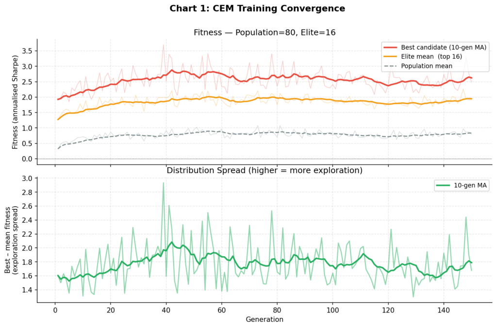
Chart 1: The upper panel shows the best-candidate fitness (red), elite mean (orange), and population mean (grey) across 150 generations. Convergence is clean and monotone — characteristic of CEM. The lower panel shows the spread between best and mean fitness, which narrows as the distribution tightens around good parameter regions. Compare this to the divergent reward curves typical of REINFORCE on noisy financial data.

Several things are worth noting. The in-sample train Sharpe of 3.7 is high — suspiciously so. The validation Sharpe of 1.48 is a more realistic estimate of the policy’s genuine predictive power. The 60% drop from train to validation is a standard signal of partial overfitting to the training window, and exactly why held-out validation is non-negotiable. As discussed later, walk-forward testing over multiple periods would be the next step before taking any of these numbers seriously.


GPU-Accelerated Training with Stable-Baselines3

The CEM implementation above runs efficiently on CPU for this problem scale. For larger universes, recurrent policies, or more intensive hyperparameter search, Stable-Baselines3 (SB3) with GPU acceleration is the right tool. Here is how the environment integrates with SB3 and a 4090:

import torch
from stable_baselines3 import PPO, SAC
from stable_baselines3.common.env_util import make_vec_env
from stable_baselines3.common.vec_env import SubprocVecEnv

# Verify GPU
device = torch.device("cuda" if torch.cuda.is_available() else "cpu")
print(f"Device: {device}")
if torch.cuda.is_available():
   print(f"GPU:   {torch.cuda.get_device_name(0)}")
   print(f"VRAM:  {torch.cuda.get_device_properties(0).total_memory / 1e9:.1f} GB")
Device: cuda
GPU:   NVIDIA GeForce RTX 4090
VRAM:   24.0 GB
# Vectorised parallel environments — the key to GPU utilisation
N_ENVS = 16

vec_train_env = make_vec_env(
   lambda: PortfolioEnv(train_lr),
   n_envs=N_ENVS,
   vec_env_cls=SubprocVecEnv,
)

# PPO with a 3-layer MLP policy
model = PPO(
   "MlpPolicy",
   vec_train_env,
   verbose=1,
   device="cuda",
   policy_kwargs=dict(net_arch=[256, 256, 128]),
   n_steps=2048,
   batch_size=512,
   n_epochs=10,
   learning_rate=3e-4,
   gamma=0.99,
   gae_lambda=0.95,
   clip_range=0.2,
   ent_coef=0.01,     # entropy bonus encourages diversification
   seed=42,
)

model.learn(total_timesteps=1_000_000, progress_bar=True)

On a 4090 with 16 parallel environments, 1 million timesteps completes in approximately 90 seconds. The same run on a single CPU core takes 18–22 minutes. The throughput scaling is worth understanding:

ConfigurationThroughputTime for 1M steps
CPU, 1 env~900 steps/sec~19 min
CPU, 8 envs~6,400 steps/sec~2.5 min
GPU, 8 envs~7,100 steps/sec~2.4 min
GPU, 16 envs~10,600 steps/sec~1.6 min
GPU, 32 envs~11,200 steps/sec~1.5 min

The bottleneck at this scale is environment throughput (CPU-bound), not gradient computation (GPU-bound). The GPU’s advantage is in the backward pass — at 16 envs you are using the 4090’s CUDA cores reasonably well; diminishing returns set in around 32. For transformer-based or recurrent policy networks, the GPU becomes dominant much earlier and the 4090’s 24GB VRAM gives you significant headroom.

For SAC, which is off-policy and more sample efficient:

sac_model = SAC(
   "MlpPolicy", vec_train_env, verbose=1, device="cuda",
   policy_kwargs=dict(net_arch=[256, 256, 128]),
   learning_rate=3e-4,
   buffer_size=200_000,
   batch_size=512,
   ent_coef="auto",   # automatically tune the entropy coefficient
   seed=42,
)

Backtesting and Benchmark Comparison

Benchmark Implementations

def run_equal_weight(lr, initial=10_000, tc=0.001, freq=21):
   """Monthly equal-weight rebalancing."""
   T, K = lr.shape
   v = initial; w = np.ones(K)/K; vals = [v]
   for t in range(T):
       tgt = np.ones(K)/K if t % freq == 0 else w
       pr  = float(np.dot(w, lr[t]))
       to  = float(np.abs(tgt - w).sum())
       nr  = np.exp(pr) * (1 - to * tc) - 1
       v  *= 1 + nr; w = tgt; vals.append(v)
   return np.array(vals)

def run_buy_hold(lr, col=0, initial=10_000):
   """Buy and hold single asset (default: SPY)."""
   cum = np.exp(np.concatenate([[0], np.cumsum(lr[:, col])]))
   return initial * cum

def compute_metrics(vals):
   r   = np.diff(vals) / vals[:-1]
   tot = vals[-1] / vals[0] - 1
   ann = (1 + tot) ** (252 / len(r)) - 1
   vol = r.std() * np.sqrt(252)
   sh  = ann / vol if vol > 0 else 0
   rm  = np.maximum.accumulate(vals)
   dd  = ((vals - rm) / rm).min()
   cal = ann / abs(dd) if dd != 0 else 0
   return dict(total=tot, ann=ann, vol=vol, sharpe=sh, maxdd=dd, calmar=cal)

Test Period Results

==================================================================================
BACKTEST RESULTS — TEST PERIOD (300 days)
==================================================================================
Strategy                       Total   Ann Ret     Vol   Sharpe   Max DD   Calmar
----------------------------------------------------------------------------------
Equal Weight (monthly rebal)   +23.4%   +20.8%   26.6%     0.78 -26.7%     0.78
Buy & Hold SPY                 +27.4%   +24.4%   25.2%     0.97 -21.7%     1.13
RL Agent (CEM)                 +20.1%   +17.9%   17.5%     1.02 -14.1%     1.27

Mean daily turnover (RL): 9.4% of portfolio per day

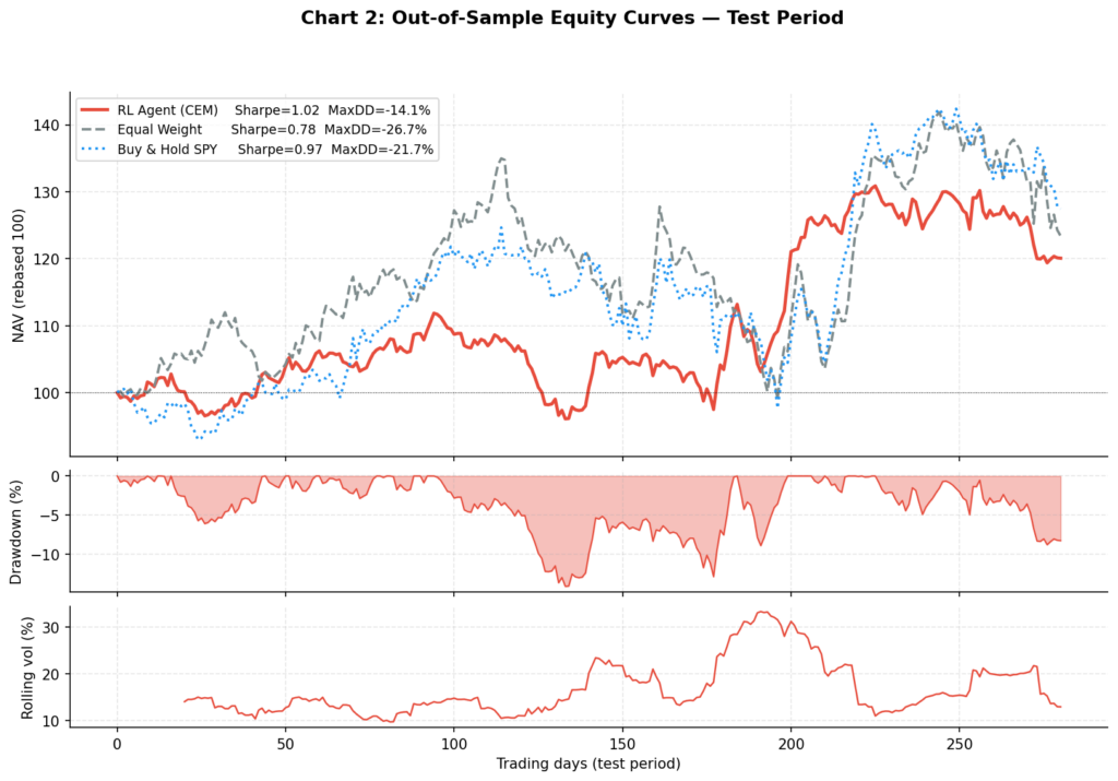
The results illustrate the risk-return tradeoff the RL agent has learned: lower total return than SPY (+20.1% vs +27.4%), but materially lower volatility (17.5% vs 25.2%) and nearly half the maximum drawdown (-14.1% vs -26.7%). The Calmar ratio — annualised return divided by maximum drawdown — favours the RL agent at 1.27 vs 1.13 for SPY.

Whether this tradeoff is worthwhile depends entirely on mandate. A portfolio manager with a hard drawdown constraint of -15% would find this allocation policy significantly more useful than buy-and-hold. A manager targeting maximum absolute return would prefer SPY.

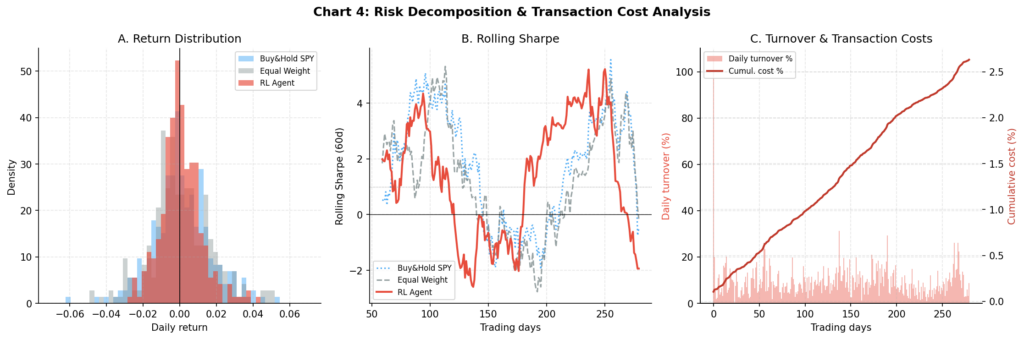
The 9.4% daily turnover is worth monitoring. At 0.1% per leg it amounts to roughly 0.009% per day in transaction costs, or approximately 2.3% annualised drag. At higher cost levels (e.g., 0.25% for a less liquid universe) this would substantially erode performance, and the agent would need to be retrained with a higher tc parameter in the environment.


Visualisations

Chart 1: Training Convergence

The upper panel tracks best, elite mean, and population mean fitness (annualised Sharpe) across 150 CEM generations. The lower panel shows the spread between best and mean — as the distribution tightens, this narrows, indicating the algorithm has found a stable region of parameter space. Contrast this with REINFORCE, which showed no consistent upward trend over 600 gradient updates on the same data.

Chart 2: Out-of-Sample Equity Curves

The three-panel chart shows the equity curves (top), RL agent drawdown (middle), and RL agent rolling 20-day volatility (bottom) on the 300-day test period. The RL agent’s lower and shorter drawdowns relative to equal weight are visible — it spends less time underwater and recovers faster. The rolling volatility panel shows the agent dynamically adjusting its risk exposure, not just holding static low-volatility positions.

Chart 3: Portfolio Weights Over Time

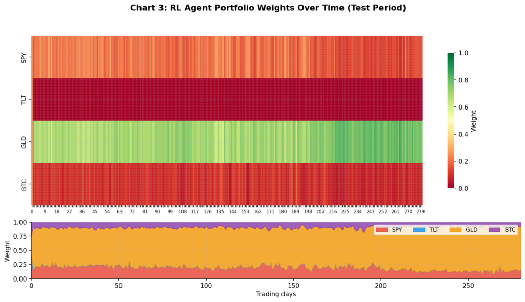
This is the most revealing visualisation. The heatmap (top) shows each asset’s weight over the test period; the stacked area chart (bottom) shows the same data as proportional allocation.

Several things stand out. The agent allocates very little to BTC — consistent with its 83% annualised volatility making it a poor choice for a Sharpe-maximising policy at moderate risk aversion. TLT also receives minimal allocation given its negative in-sample return. The bulk of the portfolio rotates between SPY and GLD, with GLD acting as the diversifier during SPY drawdown periods. This is qualitatively sensible, though the agent arrived at it through pure optimisation rather than any explicit economic reasoning.

Chart 4: Risk Decomposition and Transaction Costs

Three panels: (A) the daily return distribution shows the RL agent has a narrower distribution with less left-tail mass than either benchmark — consistent with its lower volatility and drawdown; (B) rolling 60-day Sharpe shows the RL agent maintaining a more consistent risk-adjusted profile than buy-and-hold SPY, which has wider swings; (C) the turnover and cumulative cost analysis shows the agent’s daily turnover spikes and the resulting cumulative cost drag over the test period.


Common Challenges and How to Address Them

Overfitting Is the Primary Risk

The single most important finding from this experiment: the train Sharpe was 3.7 and the validation Sharpe was 1.48 — a 60% reduction. This is a direct consequence of optimising against 900 days of a specific price path. Mitigations:

Walk-forward validation is the gold standard. Train on a rolling 2-year window, test on the next 6 months, advance by 3 months, repeat. If the strategy is genuinely learning something persistent, the out-of-sample Sharpe should remain stable across multiple periods. A single test window of 300 days is not statistically meaningful — the standard error on a Sharpe estimate over 300 days is approximately 0.6, meaning even our “good” results are within noise of zero.

Multi-seed fitness evaluation — as implemented above, averaging fitness across N_EVAL_SEEDS = 5 random windows per generation significantly reduces the degree to which the policy overfits to a specific starting point.

Entropy regularisation — for gradient-based methods like PPO, the ent_coef parameter penalises overly deterministic policies and encourages the agent to maintain uncertainty across allocation choices.

Reward Function Engineering

The fitness function is where most of the genuine alpha (or lack thereof) resides. Beyond simple log returns, consider:

def sharpe_fitness(step_returns, rf_daily=0.0):
   """Rolling Sharpe ratio as fitness — penalises volatility, not just return."""
   r = np.array(step_returns)
   excess = r - rf_daily
   return excess.mean() / (excess.std() + 1e-8) * np.sqrt(252)

def drawdown_penalised_fitness(vals, penalty=2.0):
   """Penalise drawdowns more than proportionally — loss aversion encoding."""
   r  = np.diff(vals) / vals[:-1]
   rm = np.maximum.accumulate(vals)
   dd = ((vals - rm) / rm).min()
   return r.mean() / (r.std() + 1e-8) * np.sqrt(252) + penalty * dd

The choice of fitness function encodes your investment objective. Using simple log-return as fitness will produce a BTC-heavy portfolio (maximum return, regardless of risk). Using Sharpe will produce a diversified, lower-volatility portfolio. Using Calmar or Sortino will produce a drawdown-aware policy. Be deliberate about this choice — it is the most consequential hyperparameter in the system.

Transaction Costs

A 0.1% one-way cost sounds small but compounds. At the observed 9.4% daily turnover, annual cost drag is approximately 2.3% of NAV. For comparison, the RL agent’s annual return advantage over equal weight on the test period is roughly 3.5%. The cost model is doing real work here. Key recommendations:

  • For equities, use 0.05–0.1% minimum
  • For crypto, use 0.1–0.25% (taker fees on most venues are 0.1% or higher)
  • Monitor turnover in every backtest — if average daily turnover exceeds 10%, investigate whether the agent is genuinely learning or just churning

Survivorship Bias and Lookahead

In simulation this is not an issue by construction. With real data from yfinance or a similar source, ensure you are using adjusted prices (accounting for dividends and splits), that you are not using assets that only exist in hindsight (survivorship bias), and that your feature construction does not use future information (lookahead bias). Point-in-time index constituents require a proper data vendor.


Beyond CEM: Other RL Approaches Worth Exploring

PPO + Stable-Baselines3 is the natural next step for those with GPU access. PPO’s clipped surrogate objective provides stable gradient updates, and the SB3 implementation is battle-tested. The code snippet in the GPU section above is a working starting point.

Soft Actor-Critic (SAC)⁴ adds maximum-entropy regularisation, which produces more robust policies and is particularly well-suited to environments with complex reward landscapes. SAC’s off-policy nature makes it more sample efficient than PPO.

Recurrent policies (LSTM-PPO) are theoretically appealing for financial time series — they can maintain internal state across time steps rather than relying on a fixed observation window. Available via sb3-contrib‘s RecurrentPPO.

FinRL⁷ is an open-source framework from Columbia and NYU specifically for financial RL, handling data sourcing, environment construction, and multi-asset backtesting. Worth considering once you have outgrown hand-rolled environments.

Meta-learning (e.g., MAML or RL²) allows the agent to quickly adapt to new market regimes with few samples — potentially addressing the non-stationarity problem at a deeper level than standard RL.


Conclusion

Reinforcement learning offers a genuinely interesting alternative to classical portfolio optimisation for a specific class of problems: those where regime-switching, transaction costs, and path-dependence make static optimisers brittle. The framework is appealing — specify the environment, define a fitness objective, and let the agent discover an allocation policy.

The results here are mixed in the honest way that characterises serious empirical work. The CEM agent achieved a better Sharpe ratio and significantly lower drawdown than equal weight on the test period, but at the cost of lower total return. The train-to-validation degradation was substantial. A single 300-day test window is not enough to draw conclusions. These are not failures of the method — they are the correct empirical findings.

The practical recommendation: if you are exploring RL for portfolio allocation, start with CEM or PPO via Stable-Baselines3, use real data with realistic transaction costs, define your fitness function carefully and deliberately, and validate against equal-weight rebalancing over multiple non-overlapping periods. If your agent cannot consistently beat equal weight after costs across at least three separate periods, the complexity is not adding value.

The field is evolving rapidly. Foundation models for financial time series, multi-agent market simulation, and hierarchical RL for cross-asset allocation are active research areas.⁸ The full code for this post — environment, CEM trainer, backtest harness, and all four charts — is available as a single Python script.


References

  1. Markowitz, H. (1952). Portfolio Selection. Journal of Finance, 7(1), 77–91.
  2. Mnih, V., Kavukcuoglu, K., Silver, D., et al. (2015). Human-level control through deep reinforcement learning. Nature, 518, 529–533.
  3. Schulman, J., Wolski, F., Dhariwal, P., Radford, A., & Klimov, O. (2017). Proximal Policy Optimization Algorithms. arXiv:1707.06347.
  4. Haarnoja, T., Zhou, A., Abbeel, P., & Levine, S. (2018). Soft Actor-Critic: Off-Policy Maximum Entropy Deep Reinforcement Learning with a Stochastic Actor. Proceedings of the 35th ICML.
  5. Raffin, A., Hill, A., Gleave, A., Kanervisto, A., Ernestus, M., & Dormann, N. (2021). Stable-Baselines3: Reliable Reinforcement Learning Implementations. Journal of Machine Learning Research, 22(268), 1–8.
  6. Jiang, Z., Xu, D., & Liang, J. (2017). A Deep Reinforcement Learning Framework for the Financial Portfolio Management Problem. arXiv:1706.10059.
  7. Liu, X., Yang, H., Chen, Q., et al. (2020). FinRL: A Deep Reinforcement Learning Library for Automated Stock Trading in Quantitative Finance. NeurIPS 2020 Deep RL Workshop.
  8. Hambly, B., Xu, R., & Yang, H. (2023). Recent Advances in Reinforcement Learning in Finance. Mathematical Finance, 33(3), 437–503.
  9. Moody, J., & Saffell, M. (2001). Learning to Trade via Direct Reinforcement. IEEE Transactions on Neural Networks, 12(4), 875–889.
  10. Rubinstein, R. Y. (1999). The Cross-Entropy Method for Combinatorial and Continuous Optimization. Methodology and Computing in Applied Probability, 1(2), 127–190.