Category: Factor Models

In May I published a case study on running alpha research through a team of LLM agents: four roles, instrumented handoffs, and roughly a 2× lift in hypotheses tested per week. The post was careful about what it measured. It was silent about a risk I had not thought to price.

Here is the risk. If your research agent and your competitor’s research agent are the same base model, then whatever that model believes about markets is a shared prior — and a shared prior that both of you act on is, functionally, a common factor exposure that appears in neither of your risk reports. You did not choose it. You cannot see it in your covariance matrix. And it is correlated across every firm that licensed the same weights.

That argument was given a name in May by Ye, Han, Hu and co-authors, in a paper called The Alpha Illusion [1]. Their Section 3.3 is titled “Parametric Priors as Undisclosed Implicit Factor Exposures,” and they call the mechanism parametric prior lock-in. It is a good name for a real worry, and the paper is careful enough to say what it has not done:

“We propose this as an explanatory framework rather than an established unified mechanism, called Parametric Prior Lock-in.”

Their cross-model evidence is also borrowed rather than produced: Appendix D relays bias-score gaps and view-flip rates from Lee et al. (2025), and they note that persona prompts and multi-agent debate fail to dislodge shared priors. What is missing is the specific thing a risk manager would want. They run no correlation test across model outputs, and no factor regression on generated signals. So the mechanism has a name, a plausible story, and nobody has measured whether it shows up in a book.

This post is the measurement. It is a small one, and it does not come out where I expected.

---

What I actually tested

The claim has two parts that are easy to run together and should be kept apart.

Part one, the crowding claim: independent research runs against the same model produce books that are correlated with each other.

Part two, the attribution claim: that correlation comes from the model’s weights — a shared parametric prior — rather than from something both runs are merely reading off.

Part one is worth knowing whatever the answer to part two. Part two is what makes “lock-in” a distinct phenomenon rather than a new label for an old one. Almost all of the difficulty is in part two, because the obvious confound is enormous: if four models all propose momentum and low-volatility, that may be a shared prior, or it may be that all four correctly absorbed fifty years of published asset pricing. Correlated output is the expected result here, not the finding.

So the experiment needs baselines. Two of them, fixed before I looked at anything.

The floor: random expressions

If I generate signals at random from the same vocabulary, how correlated are the resulting books? This is what “no shared anything” looks like, and it establishes that any agreement I measure is agreement at all.

The ceiling: the published canon

If eight analysts each independently built a book from the published price-based anomaly literature — momentum, reversal, low-vol, betting-against-beta, the 52-week high, idiosyncratic skewness — how correlated would their books be?

This is the baseline that matters, and it is the one the lock-in story has to beat. If eight LLM runs are no more correlated than eight literature-reading humans, then “parametric prior lock-in” has no work left to do. The crowding would be real, but it would be the crowding the anomaly literature has always produced, arriving faster.

---

Setup

Universe. Daily adjusted closes for 1,455 NASDAQ Composite constituents, 2 January 2018 to 31 May 2023, from the skfolio reference datasets [2]. The panel is fully dense — not one missing observation in 1,362 days — which is convenient and also a survivorship problem I return to below. After dropping names whose median price is under $5, 1,280 stocks remain.

The expression language. Every model gets the same restricted vocabulary: close, returns(n), logret(n), ma(n), std(n), vol(n), max_(n), min_(n), skew(n), kurt(n), beta(n), corr_mkt(n), plus delay, ts_zscore, rank, cs_zscore and simple arithmetic. Prices only. No volume, no fundamentals, no news.

Forcing every proposal into one grammar is the design decision that makes the whole thing work. Free-text research ideas cannot be compared — two people can describe the same trade in different words, or different trades in the same words. An expression can be executed. Two signals that produce the same ranking of the same stocks are the same trade, whatever their authors called them, and that is the only definition of agreement a risk manager should care about.

The syntax examples in the prompt are deliberately meaningless — ts_zscore(kurt(40), 120), abs_(logret(9)) — because my first draft used momentum and reversal as the examples, which would have seeded every model with the answer I was looking for.

Protocol. Each run receives the identical prompt and returns twelve signals, each with a name, an expression, a one-line economic rationale, and the model’s own stated confidence that the signal has positive out-of-sample IC. Eight runs: four model tiers, two independent replicates each. 96 signals, of which 95 evaluate (one produced a degenerate constant).

Scoring. Each signal becomes a dollar-neutral, rank-weighted long/short portfolio, traded with a one-day implementation lag. Each run’s twelve signals are then combined, equal-weighted on volatility-standardised returns, into a single composite book — the thing a firm would actually be running if it traded that research output. The unit of analysis is the book, not the signal, and that turns out to matter more than anything else here.

The canon control. Twelve published price-only anomalies, written in the same DSL: 12-1 momentum (Jegadeesh & Titman, 1993), one-month and one-week reversal (Jegadeesh, 1990), the low-volatility effect (Ang et al., 2006), the 52-week high (George & Hwang, 2004), betting-against-beta (Frazzini & Pedersen, 2014), the idiosyncratic-skewness effect (Boyer, Mitton & Vorkink, 2010), time-series trend (Moskowitz et al., 2012), and four variants. Eight synthetic “analysts” each draw twelve weighted picks from this literature and build a composite the same way.

---

Results

1. The crowding is real and it is large

Eight composite books built from	Mean pairwise correlation	Interval
Random expressions from the same vocabulary	+0.15	[−0.02, +0.37]
Independent LLM research runs	+0.62	[+0.54, +0.69]
The published anomaly canon	+0.82	[+0.67, +0.91]

Intervals: 5th–95th percentile of 500 control draws; for the observed value, a 21-day block-bootstrap 95% CI over 1,341 trading days.

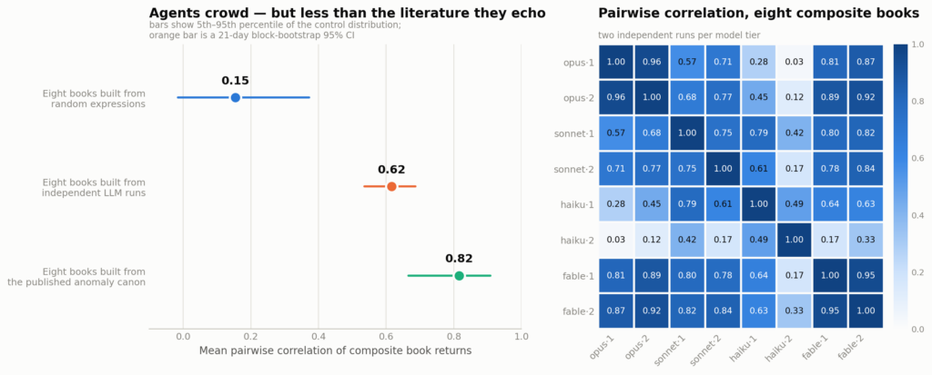
Eight independent research runs, no communication between them, produce books correlated at 0.62. Against a random-expression floor of 0.15, that is not close. If eight shops each ran this pipeline, they would be sharing something like 38% of their return variance without any of them having decided to.

The practitioner translation is the effective number of independent books, n / (1 + (n−1)ρ):

	ρ	Effective independent books (of 8)	Combined vol as % of one book
Random expressions	0.15	3.85	51%
LLM research runs	0.62	1.51	81%
Published canon	0.82	1.19	92%

Eight research agents buy you one and a half books’ worth of diversification. That is the number I would put in front of an allocator.

2. It gets worse in exactly the signals you would trade

The models each rated their own confidence in each proposal. Sorting by that self-assessment:

Model’s own stated confidence	Signals	Mean cross-run correlation
≥ 0.60	31	+0.23
0.50 – 0.60	38	+0.13
< 0.50	26	+0.06

Agreement rises monotonically with the models’ own conviction. The tail of speculative proposals is genuinely diverse; the top of the list is where everyone converges. If you filter to the ideas worth researching — which is what you would do — you are filtering toward the crowd, not away from it. Diversity in the long tail is not a hedge, because the long tail is not what gets funded.

At the concept level this is stark. Mapping each proposal to its nearest canonical anomaly:

Concept	Runs proposing it (of 8)
One-month reversal	8
One-week reversal	8
Betting-against-beta	8
Idiosyncratic-skewness effect	8
Low volatility (60d)	7
Low volatility (20d)	7
12-1 momentum	6
52-week high	6
Momentum acceleration	4
Intermediate momentum	2
Long-horizon trend	2
Path smoothness	1

Four concepts appear in every single run. Six appear in seven or more. Ninety-five distinct-looking proposals collapse to an effective rank of 4.5.

3. And yet the attribution claim fails

Here is where the post stopped being the one I set out to write.

The canon control does not come in below the LLM runs. It comes in above them, at 0.82 against 0.62. The observed value sits at the 2nd percentile of the canon control distribution.

Eight analysts independently building books out of the published anomaly literature would be more crowded than eight LLM runs were.

At the individual-signal level the same ordering holds — random expressions at +0.005, model signals at +0.12, canon signals at +0.17. On every measure I ran, the models are more diverse than the literature they are echoing, not less.

So part one of the claim survives and part two does not. The exposure is real, shared, and undisclosed. But I have no evidence it comes from the weights, and the natural alternative — the models are reproducing a low-dimensional published literature, slightly noisily — explains the data at least as well and predicts more crowding than I observed.

4. One number that looked like a finding and was not

I want to show a metric that failed, because it is the sort of thing that would have made a persuasive chart.

Regressing each model-generated signal on the twelve-signal canon basis gives a mean R² of 0.87, median 0.93, with 94% of signals above 0.5. Read naively: the models are almost entirely reproducing published anomalies.

Then run the same regression on the random expressions. Mean R² 0.83, median 0.92, 91% above 0.5.

Random noise from the same vocabulary projects onto the canon basis about as well as the models do. The metric measures the dimensionality of price-based signal space, not anything about the models. It had to be thrown away.

I mention it because this is precisely the failure mode that agentic research pipelines are good at manufacturing at scale — a plausible number, in the expected direction, that dissolves against a null nobody bothered to run. Jin Choi at Two Sigma made the same point from the other direction in January: “With AI agents, researchers can easily generate a large number of hypotheses and backtest them, which can exacerbate the overfitting issue” [3]. The binding constraint on AI-assisted research is not hypothesis generation. It is that generating hypotheses faster makes overfitting worse, not better.

5. Factor tilts

Regressing each composite book on market, momentum, short-term reversal, low-volatility and BAB legs built from the same panel:

Run	MOM	STR	LVOL	BAB	R²
opus · 1	0.25	0.29	0.11	0.19	0.81
opus · 2	0.28	0.23	0.20	0.10	0.76
sonnet · 1	0.08	0.00	0.10	0.13	0.68
sonnet · 2	0.02	0.09	0.20	0.10	0.72
haiku · 1	0.05	−0.11	0.15	0.03	0.57
haiku · 2	0.04	−0.17	−0.15	0.15	0.66
fable · 1	0.26	0.13	0.27	0.04	0.73
fable · 2	0.22	0.14	0.19	0.17	0.80

72% of individual signals have a factor R² above 0.5. Mean annualised alpha to this five-factor set is 1.2%, and fewer than half the signals have positive alpha at all. Whatever these agents are producing, most of it is factor exposure wearing a new name — which is a finding about disclosure, and survives the collapse of the lock-in attribution intact. A book you cannot decompose is a book whose risk you are not reporting.

Note also that the tilts are not a shared direction: mean cosine similarity between run-level tilt vectors is +0.10. The runs agree on which anomalies exist far more than they agree on how to weight them.

6. The one hint that the weights matter

Sorting composite-book pairs by whether they came from the same model tier:

	Pairs	Mean correlation
Same tier (two runs of the same model)	4	+0.79
Different tier	24	+0.59

That is the right shape for a dose-response on shared weights. It is also four data points, all within a single model family, and I would not defend it further than “worth running properly.”

---

What this does and does not show

It shows that independent research runs against LLMs produce composite books correlated at 0.62 — four times the random-expression floor — that the agreement concentrates in the highest-conviction proposals, that four canonical anomalies appeared in all eight runs, and that roughly three-quarters of the resulting signals are explicable as factor exposure.

It does not show parametric prior lock-in. On the only test I could construct for it, the published literature produces more crowding than the models did.

The limitations that matter most, in order:

All eight runs are from one model family. This is the big one. The tier contrast — opus, sonnet, haiku, fable — is a within-family proxy and cannot separate “shared weights” from “shared literature,” because these models share both. The decisive experiment is cross-family: identical prompts against models from genuinely different pretraining lineages, testing whether within-family agreement exceeds cross-family agreement. I could not run it here for want of API access to the other providers. The code is written and the harness is the same; this is a gap, not a design choice, and until someone runs it the lock-in hypothesis is neither supported nor refuted — only unmeasured.

Eight runs is not a cross-section. Four tiers, two replicates. Every interval in this post is wide, and the same-tier contrast rests on four pairs.

The DSL constrains the space, and I cannot sign the bias. Price-only signals live in a low-dimensional space, which mechanically raises agreement; but the restriction applies equally to the canon control, which is the comparison that carries the argument.

The canon control is my list. Twelve anomalies I chose. A longer or differently-weighted canon moves the 0.82. I would treat the ordering of the three baselines as the result and the levels as approximate.

The performance numbers are not tradeable. Daily rebalancing, gross of costs, on a dollar-neutral book. The 1.68 Sharpe on one-week reversal in the canon set is a well-known cost-eaten effect and appears here only as a benchmark component.

The panel is survivorship-clean in the worst way. skfolio documents nothing about how its 1,455 names were selected, but the panel’s complete absence of missing observations over five and a half years implies the universe is survivorship-conditioned by construction: delisted, acquired and bankrupt NASDAQ names from that window cannot be in it. The documentation is also explicit that this is “a stale dataset… not intended for investment, trading, or commercial use.” That biases the level of every backtest here. It does not obviously bias the correlation comparisons, which are all run on the same panel, but I would not swear to it. A serious version of this experiment runs on a point-in-time universe.

Model versions are a moving target. This is a snapshot of specific checkpoints in August 2026. Re-run it in six months and the numbers will differ; that is a property of the object being measured, not a defect in the measurement.

---

What I think is actually going on

The crowding is real and I would now treat it as a risk to be measured. But “parametric prior lock-in” is the wrong mental model for it, at least on this evidence.

The better model is duller and more actionable: an LLM is a fast, lossy index of the published anomaly literature. Ask it for signals and you get the canon back, sampled with noise, weighted by whatever the training corpus emphasised. The crowding does not originate in the weights. It originates in the fact that the published cross-sectional anomaly literature is itself extremely low-dimensional — twelve canonical signals with an effective rank of 2.6 — and has been the common input to systematic equity research for thirty years.

Which means the honest version of the warning is not “beware the model’s hidden priors.” It is: the tool makes it much cheaper to rediscover what everyone already knows, and it will do so with great fluency and a plausible economic rationale attached to each one.

McLean and Pontiff put numbers on what that costs [4]. Across 97 published predictors, returns are 26% lower out-of-sample — their upper bound on data mining in the original studies — and 58% lower post-publication. The difference, 32%, is the decay attributable to publication-informed trading: the part caused by other people reading the same paper and putting it on. That is the number that bites here, because an agent that reliably rediscovers published anomalies is an agent that reliably rediscovers decayed ones, and writes you a confident paragraph about the mechanism while doing it.

Their paper also contains a finding I did not expect to need: predictor portfolios show post-publication increases in correlation with other published-predictor portfolios. The literature does not merely decay after publication — it converges. That is the 0.82 canon number arriving from a completely independent direction, twenty years of data earlier.

That is a different failure than the one the Alpha Illusion paper is pointing at, and in some ways a worse one, because it is not exotic. It does not need a story about weight-sharing across firms. It only needs the thing we already knew about the anomaly literature, plus a tool that samples from it at essentially zero marginal cost.

There is also a mildly contrarian note in the data that I want to state plainly rather than bury: on every measure I ran, the models were more diverse than the literature. If your prior was that LLMs homogenise research relative to a room of well-read humans, this small experiment points the other way.

Where to take this next

1. The cross-family arm. Same prompts, models from different pretraining lineages. Does within-family agreement exceed cross-family agreement once “family” means something? This is the experiment that settles it, and it is a few hundred dollars of API.
2. A human control arm. Give the same prompt and the same DSL to a dozen quant researchers. If humans come in at 0.6 too, the whole topic is a non-story about tools and a real story about the literature.
3. Adversarial evidence. Feed a model data that should flip a tilt and see whether the prior holds anyway. Agreement is not lock-in; persistence against contrary evidence is, and it is the one test that would distinguish them.
4. Widen the vocabulary. Volume, fundamentals, and cross-sectional interactions raise the dimensionality of the space. If agreement survives a richer DSL, it is a stronger result; if it collapses, the price-only constraint was doing the work.
5. Novelty-conditioned generation. Ask explicitly for signals not in the published literature and re-run the whole comparison. My guess, worth about as much as any guess, is that the agreement falls and the alpha falls further.

---

References

[1] Ye, Han, Hu, Bu, Chen, Wen, Mandic, Sun, Yinghui & Xu, The Alpha Illusion: Reported Alpha from LLM Trading Agents Should Not Be Treated as Deployment Evidence, arXiv:2605.16895, 16 May 2026. The TradingAgents Sharpe degradation from 0.43 to 0.22 under realistic frictions is their own result, from a one-year, five-ticker reproduction (Figure 1, setup in Appendix B). The frequently-quoted 71.85% post-cutoff drop in FinMem returns is not theirs — it is their citation to Li et al. (2025).

[2] skfolio, load_nasdaq_dataset — daily adjusted closes for 1,455 NASDAQ Composite constituents, 2018-01-02 to 2023-05-31. https://skfolio.org/generated/skfolio.datasets.load_nasdaq_dataset.html

[3] Jin Choi, Head of Technique Forecasting, in Two Sigma, AI in Investment Management: 2026 Outlook (Part II), 21 January 2026. https://www.twosigma.com/articles/ai-in-investment-management-2026-outlook-part-ii/

[4] McLean & Pontiff, Does Academic Research Destroy Stock Return Predictability?, Journal of Finance 71(1), 2016. 97 predictors from 80 studies.

[5] Harvey, Liu & Zhu, …and the Cross-Section of Expected Returns, Review of Financial Studies, 2016.

[6] Bailey & López de Prado, The Deflated Sharpe Ratio, Journal of Portfolio Management, 2014.

[7] Jegadeesh & Titman, Returns to Buying Winners and Selling Losers, JF 48(1), 1993 — the 12-1 skip-a-month construction is Carhart (1997); Jegadeesh, JF 45(3), 1990; Ang, Hodrick, Xing & Zhang, JF 61(1), 2006; George & Hwang, JF 59(5), 2004; Frazzini & Pedersen, JFE 111(1), 2014; Boyer, Mitton & Vorkink, Expected Idiosyncratic Skewness, RFS 23(1), 2010; Moskowitz, Ooi & Pedersen, JFE 104(2), 2012.

---

Code and data

The full pipeline is four files — signal_dsl.py (grammar and portfolio construction), canon.py (the twelve published anomalies), prompt.md (the frozen prompt), evaluate.py (scoring and controls). Both datasets are public and fetched by URL. It runs in about three minutes on a laptop, with fixed seeds and pinned model versions.

The one thing I would ask of anyone re-running it: run the random-expression null first. It cost me the most persuasive number in the post, which is exactly what a null is for.

---

"""
evaluate.py — turn every generated signal into a return stream, then measure
(a) cross-model agreement and (b) factor tilts.
"""
import json, glob, os, itertools
import numpy as np
import pandas as pd
from signal_dsl import Ctx, evaluate, ls_returns, to_weights
from canon import CANON

RUNS = {  # run id -> (family, model tier)
    "A1": ("anthropic", "opus"),   "A2": ("anthropic", "opus"),
    "B1": ("anthropic", "sonnet"), "B2": ("anthropic", "sonnet"),
    "C1": ("anthropic", "haiku"),  "C2": ("anthropic", "haiku"),
    "D1": ("anthropic", "fable"),  "D2": ("anthropic", "fable"),
}


def load_panel(path="data/prices.pkl", min_price=5.0):
    px = pd.read_pickle(path)
    px = px.loc[:, px.median() >= min_price]
    return px


def build(ctx, items, tag):
    """Evaluate a dict/list of {name, expr} into return streams. Returns (rets, sigs, errors)."""
    rets, sigs, errs = {}, {}, []
    for it in items:
        key = f"{tag}:{it['name']}"
        try:
            s = evaluate(it["expr"], ctx)
            r = ls_returns(s, ctx)
            if r.std() == 0 or len(r) < 400:
                errs.append((key, "degenerate"))
                continue
            rets[key] = r
            sigs[key] = s
        except Exception as e:  # noqa: BLE001
            errs.append((key, repr(e)[:90]))
    return rets, sigs, errs


def mean_xs_rank_corr(s1, s2, sample_every=5):
    """Average cross-sectional Spearman correlation between two signal frames."""
    idx = s1.index.intersection(s2.index)[::sample_every]
    out = []
    for d in idx:
        a, b = s1.loc[d], s2.loc[d]
        m = a.notna() & b.notna() & np.isfinite(a) & np.isfinite(b)
        if m.sum() < 50:
            continue
        c = a[m].rank().corr(b[m].rank())
        if np.isfinite(c):
            out.append(c)
    return float(np.mean(out)) if out else np.nan


def effective_rank(R):
    """Participation ratio of the correlation-matrix eigenvalue spectrum."""
    C = R.corr().values
    C = np.nan_to_num(C, nan=0.0)
    w = np.linalg.eigvalsh(C)
    w = np.clip(w, 0, None)
    return float(w.sum() ** 2 / (w ** 2).sum())


def main():
    px = load_panel()
    ctx = Ctx(px)
    print(f"universe: {px.shape[1]} names, {px.shape[0]} days, "
          f"{px.index.min().date()} to {px.index.max().date()}")

    # --- canon control arm ---
    canon_r, canon_s, canon_e = build(ctx, [{"name": k, "expr": v} for k, v in CANON.items()], "CANON")
    print(f"canon: {len(canon_r)} usable, errors={canon_e}")

    # --- model arms ---
    all_r, all_s, meta = {}, {}, {}
    for run in sorted(RUNS):
        items = json.load(open(f"gen/{run}.json"))
        r, s, e = build(ctx, items, run)
        all_r.update(r); all_s.update(s)
        for k in r:
            meta[k] = RUNS[run]
        print(f"{run} ({RUNS[run][1]:6s}): {len(r):2d}/12 usable" + (f"  errors={e}" if e else ""))

    R = pd.DataFrame(all_r).dropna(how="all")
    R.to_pickle("data/model_returns.pkl")
    CR = pd.DataFrame(canon_r).dropna(how="all")
    with open("data/meta.json", "w") as f:
        json.dump({k: list(v) for k, v in meta.items()}, f)

    keys = list(R.columns)

    # ---------------- agreement on return streams ----------------
    rc = R.corr()
    within_tier, cross_tier, all_pairs = [], [], []
    for a, b in itertools.combinations(keys, 2):
        if a.split(":")[0][0] == b.split(":")[0][0]:   # same model tier
            within_tier.append(rc.loc[a, b])
        else:
            cross_tier.append(rc.loc[a, b])
        all_pairs.append(rc.loc[a, b])

    cc = CR.corr()
    canon_pairs = [cc.loc[a, b] for a, b in itertools.combinations(CR.columns, 2)]

    print("\n=== RETURN-STREAM CORRELATION ===")
    for nm, v in [("model x model (all)", all_pairs),
                  ("  same tier", within_tier),
                  ("  different tier", cross_tier),
                  ("canon x canon (control)", canon_pairs)]:
        v = np.array(v)
        print(f"{nm:26s} n={len(v):5d}  mean={v.mean():+.3f}  median={np.median(v):+.3f}  "
              f"|r|>0.5: {(np.abs(v) > 0.5).mean() * 100:5.1f}%")

    print(f"\neffective rank: models {effective_rank(R):.2f} of {R.shape[1]} signals")
    print(f"effective rank: canon  {effective_rank(CR):.2f} of {CR.shape[1]} signals")

    # ---------------- nearest-canon projection ----------------
    print("\n=== HOW MUCH OF EACH MODEL SIGNAL IS ALREADY IN THE CANON ===")
    common = R.index.intersection(CR.index)
    X = CR.loc[common].fillna(0.0).values
    X = np.column_stack([np.ones(len(X)), X])
    r2s, best = {}, {}
    for k in keys:
        y = R.loc[common, k].fillna(0.0).values
        coef, *_ = np.linalg.lstsq(X, y, rcond=None)
        resid = y - X @ coef
        r2 = 1 - resid.var() / y.var() if y.var() > 0 else np.nan
        r2s[k] = r2
        cors = {c: abs(R.loc[common, k].corr(CR.loc[common, c])) for c in CR.columns}
        best[k] = max(cors, key=cors.get)
    r2v = np.array(list(r2s.values()))
    print(f"R^2 of model signal on canon basis: mean={np.nanmean(r2v):.3f} "
          f"median={np.nanmedian(r2v):.3f}  >0.5: {(r2v > 0.5).mean() * 100:.1f}%")

    pd.Series(r2s).sort_values(ascending=False).to_csv("data/canon_r2.csv")
    pd.Series(best).to_csv("data/nearest_canon.csv")

    # ---------------- factor tilts ----------------
    print("\n=== FACTOR TILTS ===")
    F = pd.DataFrame({
        "MKT":  ctx.ret1.mean(axis=1),
        "MOM":  canon_r["CANON:mom_12_1"],
        "STR":  canon_r["CANON:reversal_1m"],
        "LVOL": canon_r["CANON:low_vol_60"],
        "BAB":  canon_r["CANON:bab"],
    }).dropna()
    F.to_pickle("data/factors.pkl")

    rows = []
    for k in keys:
        d = pd.concat([R[k], F], axis=1).dropna()
        if len(d) < 300:
            continue
        y = d.iloc[:, 0].values
        Xf = np.column_stack([np.ones(len(d)), d.iloc[:, 1:].values])
        coef, *_ = np.linalg.lstsq(Xf, y, rcond=None)
        resid = y - Xf @ coef
        r2 = 1 - resid.var() / y.var()
        rows.append(dict(signal=k, family=meta[k][0], tier=meta[k][1],
                         alpha_ann=coef[0] * 252, MKT=coef[1], MOM=coef[2],
                         STR=coef[3], LVOL=coef[4], BAB=coef[5], r2=r2))
    T = pd.DataFrame(rows).set_index("signal")
    T.to_csv("data/tilts.csv")
    print(T[["MKT", "MOM", "STR", "LVOL", "BAB", "r2"]].describe().loc[["mean", "50%", "std"]].round(3))
    print(f"\nshare of model signals with factor R^2 > 0.5: "
          f"{(T.r2 > 0.5).mean() * 100:.1f}%")
    print(f"median |STR| beta: {T.STR.abs().median():.3f}   "
          f"median |MOM| beta: {T.MOM.abs().median():.3f}")

    # tilt-vector agreement
    V = T[["MKT", "MOM", "STR", "LVOL", "BAB"]]
    Vn = V.div(np.linalg.norm(V.values, axis=1), axis=0)
    S = Vn.values @ Vn.values.T
    iu = np.triu_indices_from(S, 1)
    print(f"cosine similarity of tilt vectors: mean={S[iu].mean():+.3f} "
          f"median={np.median(S[iu]):+.3f}")

    return R, CR, T


if __name__ == "__main__":
    main()

"""
signal_dsl.py — a restricted expression language for cross-sectional equity signals,
plus an evaluator that turns any expression into a dollar-neutral long/short return stream.

Every model in the experiment sees the SAME vocabulary and the SAME data, so any
disagreement in output is disagreement about ideas, not about tooling.

Data: daily adjusted closes, wide (dates x tickers).
"""
from __future__ import annotations
import numpy as np
import pandas as pd

# ----------------------------------------------------------------------------
# Primitives. Each returns a DataFrame aligned to (dates x tickers).
# ----------------------------------------------------------------------------

class Ctx:
    def __init__(self, px: pd.DataFrame):
        self.px = px
        self.ret1 = px.pct_change()

    # --- raw ---
    @property
    def close(self):
        return self.px

    # --- returns ---
    def returns(self, n: int):
        """Simple return over the trailing n days."""
        return self.px.pct_change(n)

    def logret(self, n: int = 1):
        return np.log(self.px).diff(n)

    # --- rolling time-series stats ---
    def ma(self, n: int):
        return self.px.rolling(n).mean()

    def std(self, n: int):
        """Rolling std of daily returns."""
        return self.ret1.rolling(n).std()

    def vol(self, n: int):
        """Annualised rolling volatility."""
        return self.ret1.rolling(n).std() * np.sqrt(252)

    def max_(self, n: int):
        return self.px.rolling(n).max()

    def min_(self, n: int):
        return self.px.rolling(n).min()

    def skew(self, n: int):
        return self.ret1.rolling(n).skew()

    def kurt(self, n: int):
        return self.ret1.rolling(n).kurt()

    def delay(self, x, n: int):
        return _df(x).shift(n)

    def ts_zscore(self, x, n: int):
        x = _df(x)
        m = x.rolling(n).mean()
        s = x.rolling(n).std()
        return (x - m) / s.replace(0.0, np.nan)

    def beta(self, n: int):
        """Rolling beta of each stock to the equal-weighted panel."""
        mkt = self.ret1.mean(axis=1)
        cov = self.ret1.rolling(n).cov(mkt)
        var = mkt.rolling(n).var()
        return cov.div(var, axis=0)

    def corr_mkt(self, n: int):
        mkt = self.ret1.mean(axis=1)
        return self.ret1.rolling(n).corr(mkt)

    # --- cross-sectional ---
    def rank(self, x):
        """Cross-sectional rank scaled to [0, 1]."""
        return _df(x).rank(axis=1, pct=True)

    def cs_zscore(self, x):
        x = _df(x)
        return x.sub(x.mean(axis=1), axis=0).div(x.std(axis=1).replace(0.0, np.nan), axis=0)

    def neg(self, x):
        return -_df(x)

    def log(self, x):
        return np.log(_df(x).where(lambda d: d > 0))

    def abs_(self, x):
        return _df(x).abs()

    def sign(self, x):
        return np.sign(_df(x))

    def clip(self, x, lo, hi):
        return _df(x).clip(lo, hi)


def _df(x):
    return x if isinstance(x, pd.DataFrame) else x


ALLOWED = [
    "close", "returns", "logret", "ma", "std", "vol", "max_", "min_", "skew", "kurt",
    "delay", "ts_zscore", "beta", "corr_mkt", "rank", "cs_zscore", "neg", "log",
    "abs_", "sign", "clip",
]


def make_namespace(ctx: Ctx) -> dict:
    ns = {}
    for name in ALLOWED:
        attr = getattr(ctx, name)
        ns[name] = attr
    ns["np"] = np
    return ns


def evaluate(expr: str, ctx: Ctx) -> pd.DataFrame:
    """Evaluate a DSL expression to a (dates x tickers) signal frame."""
    ns = make_namespace(ctx)
    out = eval(expr, {"__builtins__": {}}, ns)  # noqa: S307 - restricted namespace
    if not isinstance(out, pd.DataFrame):
        raise TypeError(f"expression returned {type(out)}, expected DataFrame")
    return out


# ----------------------------------------------------------------------------
# Portfolio construction
# ----------------------------------------------------------------------------

def to_weights(sig: pd.DataFrame, min_names: int = 50) -> pd.DataFrame:
    """
    Dollar-neutral, rank-weighted cross-sectional portfolio.
    Weights sum to zero each day and have gross exposure of 1.
    """
    s = sig.replace([np.inf, -np.inf], np.nan)
    valid = s.notna().sum(axis=1)
    r = s.rank(axis=1, pct=True)
    w = r.sub(r.mean(axis=1), axis=0)
    gross = w.abs().sum(axis=1).replace(0.0, np.nan)
    w = w.div(gross, axis=0)
    w = w.where(valid.ge(min_names), np.nan)
    return w


def ls_returns(sig: pd.DataFrame, ctx: Ctx, lag: int = 1) -> pd.Series:
    """
    Long/short return stream. Signal at t is traded into t+lag, so there is
    no same-bar look-ahead.
    """
    w = to_weights(sig).shift(lag)
    r = ctx.ret1
    common = w.index.intersection(r.index)
    out = (w.loc[common] * r.loc[common]).sum(axis=1, skipna=True)
    out[w.loc[common].isna().all(axis=1)] = np.nan
    return out.dropna()


def rank_ic(sig: pd.DataFrame, ctx: Ctx, horizon: int = 21) -> pd.Series:
    """Daily cross-sectional Spearman IC against forward `horizon`-day returns."""
    fwd = ctx.px.pct_change(horizon).shift(-horizon)
    s = sig.replace([np.inf, -np.inf], np.nan)
    ics = {}
    for d in s.index:
        a = s.loc[d]
        b = fwd.loc[d] if d in fwd.index else None
        if b is None:
            continue
        m = a.notna() & b.notna()
        if m.sum() < 50:
            continue
        ics[d] = a[m].rank().corr(b[m].rank())
    return pd.Series(ics).dropna()