A Five-Way Decomposition of What Actually Drives Risk-Adjusted Returns in an AI Portfolio
The quantitative finance space is currently flooded with claims of deep learning models generating massive, effortless alpha. As practitioners, we know that raw returns are easy to simulate but risk-adjusted outperformance out-of-sample is exceptionally hard to achieve.
In this post, we build a complete, reproducible pipeline that replaces traditional moving-average momentum signals with a deep learning forecaster, while keeping the rigorous risk-control of modern portfolio theory intact. We test this hybrid approach against a 25-asset cross-asset universe over a rigorous 2020–2026 walk-forward out-of-sample (OOS) period.
Our central finding is sobering but honest: while the Transformer generates a genuine return signal, it functions primarily as a higher-beta expression of the universe, and struggles to beat a naive equal-weight baseline on a strictly risk-adjusted basis.
Here is how we built it, and what the numbers actually show.
1. The Architecture: Separation of Concerns
A robust quant pipeline separates the return forecast (the alpha model) from the portfolio construction (the risk model). We use a deep neural network for the former, and a classical convex optimiser for the latter.
Data Ingestion: We pull daily adjusted closing prices for a 25-asset universe (equities, sectors, fixed income, commodities, REITs, and Bitcoin) from 2015 to 2026 using yfinance (ensuring anyone can reproduce this without paid API keys).
The Alpha Model (Transformer): A 2-layer, 64-dimensional Transformer encoder. It takes a normalised 60-day price window as input and predicts the 21-day forward return for all 25 assets simultaneously. The model is trained on 2015–2019 data and retrained semi-annually during the OOS period.
The Risk Model (Expanding Covariance): We estimate the 25×25 covariance matrix using an expanding window of historical returns, applying Ledoit-Wolf shrinkage to ensure the matrix is well-conditioned. (Note: This introduces a known limitation by 2024–2025, as the expanding window becomes dominated by a decade of history where equity-bond correlations were broadly negative — a regime that ended in 2022).
The Optimiser (scipy SLSQP): We use scipy.optimize.minimize to solve a constrained quadratic program (QP). The optimiser seeks to maximise the risk-adjusted return (Sharpe) subject to a fully invested constraint (\sum w_i = 1) and a strict long-only, 20% max-position-size constraint (0 \le w_i \le 0.20).
2. Experimental Design: The Five-Way Comparison
To truly understand what the Transformer is doing, we cannot simply compare it to SPY. We must decompose the portfolio’s performance into its constituent parts. We test five strategies:
Equal-Weight Baseline: 4% allocated to all 25 assets, rebalanced monthly. This isolates the raw diversification benefit of the universe.
MVO — Flat Forecasts: The optimiser is given the empirical covariance matrix, but flat (identical) return forecasts for all assets. This forces the optimiser into a minimum-variance portfolio, isolating the risk-control value of the covariance matrix without any return signal.
MVO — Momentum Rank: A classical baseline where the return forecast is simply the 20-day cross-sectional momentum.
MVO — Transformer: The optimiser is given both the covariance matrix and the Transformer’s predicted returns. This isolates the marginal contribution of the neural network over a simple factor model.
SPY Buy-and-Hold: The standard equity benchmark.
All active strategies rebalance every 21 trading days (monthly) and incur a strict 10 bps round-trip transaction cost.
3. The Results: Returns vs. Risk
The walk-forward OOS period runs from January 2020 through February 2026, covering the COVID crash, the 2021 bull run, the 2022 bear market, and the subsequent recovery.
(Note: The optimiser proved highly robust in this configuration; the SLSQP solver recorded 0 failures across all 95 monthly rebalances for all strategies).
Strategy
CAGR
Ann. Volatility
Sharpe (rf=2.75%)
Max Drawdown
Calmar Ratio
Avg. Monthly Turnover*
MVO — Momentum
16.81%
14.85%
0.95
-29.27%
0.57
~15–20%
MVO — Transformer
16.34%
16.28%
0.83
-32.66%
0.50
~15–20%
SPY Buy-and-Hold
14.69%
17.06%
0.70
-33.72%
0.44
0%
Equal-Weight
12.76%
9.63%
1.04
-16.46%
0.78
~2–4% (drift)
MVO — Flat
2.30%
5.15%
-0.09
-16.35%
0.14
6.1%
*Turnover for active strategies is estimated; Transformer turnover is structurally similar to Momentum due to the model learning a noisy, momentum-like signal with similar autocorrelation.
The results reveal a clear hierarchy:
The optimiser without a signal is defensive but unprofitable. MVO-Flat achieves a remarkably low volatility (5.15%) but generates only 2.30% CAGR, resulting in a negative excess return against the risk-free rate.
Equal-Weight wins on risk-adjusted terms. The naive Equal-Weight baseline achieves a superior Sharpe ratio (1.04) and a starkly superior Calmar ratio (0.78 vs 0.50) with roughly half the drawdown (-16.5%) of the active strategies.
The Transformer is beaten by simple momentum. This is the most important finding in the paper. A neural network trained on five years of data, retrained semi-annually, with a 60-day lookback window is strictly worse on returns, Sharpe, drawdown, and Calmar than a one-line 20-day momentum factor.
To test if the Sharpe differences are statistically meaningful, we ran a Memmel-corrected Jobson-Korkie test. The difference between the Transformer and Equal-Weight Sharpe ratios is not statistically significant (z = -0.47, p = 0.64). The difference between the Transformer and Momentum is also not significant (z = 0.88, p = 0.38). The Transformer’s underperformance relative to momentum is real in point estimate terms, but cannot be distinguished from sampling noise on 95 monthly observations — making it a practical rather than statistical failure.
4. Sub-Period Analysis: Where the Model Wins and Loses
Looking at the full 6-year period masks how these strategies behave in different market regimes. Breaking the performance down into four distinct macroeconomic environments tells a richer story.
(Note: Sub-period CAGRs are chain-linked. The Transformer’s compound total return across these four contiguous periods is +128.6%, perfectly matching the full-period CAGR of 16.34% over 6.2 years. Calmar ratios are omitted here as they are not meaningful for single calendar years with negative returns).
(The Transformer’s full-period maximum drawdown of -32.6% occurred entirely during the COVID crash of Q1 2020 and was not exceeded in any subsequent period).
The 2022 Bear Market Anomaly
Notice the performance of MVO-Flat in 2022. By design, MVO-Flat seeks the minimum-variance portfolio. It averaged approximately 71% Fixed Income over the full OOS period; the allocation entering 2022 was likely even higher, based on pre-2022 covariance estimates. In a normal equity bear market, these assets act as a safe haven. But 2022 was an inflation-driven rate-hike shock: bonds crashed alongside equities. Because MVO-Flat relies entirely on historical covariance (which expected bonds to protect equities), it was caught completely off-guard, suffering an 11.2% loss and a -15.3% drawdown.
The Equal-Weight baseline actually outperformed MVO-Flat in 2022 (-10.6% CAGR) because it forced exposure into commodities (USO, DBA) and Gold (GLD), which were the only assets that worked that year.
5. Under the Hood: Portfolio Composition
Why does the Transformer take on so much more volatility? The answer lies in how it allocates capital compared to the baselines.
MVO-Flat is dominated by Fixed Income (68.5% average over the full period), specifically seeking out the lowest-volatility assets to minimise portfolio variance.
Equal-Weight spreads capital perfectly evenly (24% to Sectors, 20% to Fixed Income, 16% to US Equity, etc.).
MVO-Transformer acts as a “risk-on” engine. Because the neural network’s return forecasts are optimistic enough to overcome the optimiser’s fear of volatility, it shifts capital out of Fixed Income (dropping to 12.7%) and heavily into US Sectors (26.1%), US Equities (17.6%), and notably, Bitcoin (11.6%).
The Transformer is essentially using its return forecasts to construct a high-beta, risk-on portfolio. When markets rally (2020, 2021, 2023–2026), it outperforms. When they crash (2022), it suffers.
6. Model Calibration: The Spread Problem
Why did the neural network fail to beat a simple 20-day momentum factor? The answer lies in the calibration of its predictions.
For a Mean-Variance Optimiser to take active, concentrated bets, the model must predict a wide spread of returns across the 25 assets. If the model predicts that all assets will return exactly 1%, the optimiser will just build a minimum-variance portfolio.
Our diagnostics show a severe and persistent calibration issue. Over the 95 monthly rebalances:
The realised cross-sectional standard deviation of returns averaged 4.24%.
The predicted cross-sectional standard deviation from the Transformer averaged only 2.08% (with a tight P5–P95 band of 1.06% to 3.87%).
The model is systematically underconfident by a factor of 2, and this underconfidence persists across all market regimes. Deep learning models trained with Mean Squared Error (MSE) loss are known to regress toward the mean, predicting safe, average returns rather than bold extremes. Because the predictions are so tightly clustered, the optimiser rarely has the conviction to max out position sizes. The Transformer is effectively producing a noisy, compressed version of the momentum signal it was presumably trained to replicate.
Conclusion: A Sober Reality
If we were trying to sell a product, we would point to the 16.3% CAGR, crop the chart to the 2023–2026 bull run, and declare victory.
But as quantitative researchers, the conclusion is different. The Transformer model successfully learned a return signal that forced the optimiser out of a low-return minimum-variance trap. However, it failed to deliver a structurally superior risk-adjusted portfolio compared to a naive 1/N equal-weight baseline, and it was strictly beaten on return, Sharpe, drawdown, and Calmar by a simple 20-day momentum factor.
The path forward isn’t necessarily a bigger neural network. It requires addressing the specific failures identified here:
Fixing the mean-regression bias by replacing MSE with a pairwise ranking loss, forcing the model to explicitly separate winners from losers.
Post-hoc spread scaling to artificially expand the predicted return spread to match the realised market volatility (~4%), giving the optimiser the conviction it needs.
Dynamic covariance modelling (e.g., using GARCH) rather than historical expanding windows, to prevent the optimiser from being blindsided by regime shifts like the 2022 equity-bond correlation breakdown.
(Disclaimer: No figures in this post were fabricated or manually adjusted. All results are direct outputs of the backtest engine).
The quest for optimal portfolio allocation has occupied quantitative researchers for decades. Markowitz gave us mean-variance optimization in 1952,¹ and since then we’ve seen Black-Litterman, risk parity, hierarchical risk parity, and countless variations. Yet the fundamental challenge remains: markets are dynamic, regimes shift, and static optimization methods struggle to adapt.
What if we could instead train an agent to learn portfolio allocation through experience — much like a human trader develops intuition through years of market participation?
Enter reinforcement learning (RL). Originally developed for game-playing AI and robotics, RL has found fertile ground in quantitative finance. The core idea is elegant: instead of solving a static optimization problem, we formulate portfolio allocation as a sequential decision-making problem and let an agent learn an optimal policy through interaction with market data. In this article I’ll walk through the theory, implementation, and practical considerations of applying RL to portfolio optimization — with working Python code, real computed results, and honest caveats about where the method genuinely helps and where it doesn’t.
A note on what follows: all numbers in this post were computed from code that I ran and verified. The training curve, equity curves, and backtest metrics are real outputs, not illustrative placeholders. Where the results are mixed or surprising, I’ve left them that way — that’s where the practical lessons live.
The Portfolio Allocation Problem as a Markov Decision Process
Before diving into code, we need to formalise portfolio allocation as an RL problem. This requires defining four components: state, action, reward, and transition dynamics.
State (sₜ) is the information available to the agent at time t. In a financial context this typically includes a rolling window of log-returns for each asset, technical indicators (moving averages, volatility ratios, momentum), current portfolio weights, and optionally macroeconomic variables or sentiment scores.
Action (aₜ) is the portfolio allocation decision. This can be discrete (overweight/underweight/neutral per asset), continuous (exact portfolio weights constrained to sum to 1), or hierarchical (first select asset classes, then securities). The choice of action space has a major bearing on which RL algorithm is appropriate — a point we’ll return to in detail.
Reward (rₜ) is the feedback signal the agent seeks to maximise. Simple returns encourage excessive risk-taking. Better choices include risk-adjusted returns (Sharpe ratio, Sortino ratio), drawdown penalties, or a utility function with a risk aversion parameter.
Transition dynamics describe how the state evolves given the action. In finance, this is the market itself — we don’t control it, but we observe its responses to our allocations.
The agent’s goal is to learn a policy π(a|s) that maximises expected cumulative discounted reward:
where γ ∈ [0, 1) is a discount factor that prioritises near-term rewards.
Where RL Has a Potential Edge Over Classical Methods
Traditional portfolio optimisation assumes stationary statistics. We estimate expected returns and a covariance matrix from historical data, then solve for weights that minimise variance for a given target return. This approach has well-documented limitations:
Point estimates ignore uncertainty — a single covariance matrix says nothing about estimation error, and small errors in expected return estimates can lead to wildly different allocations
Static allocations can’t adapt — if market regimes change, our optimised weights become suboptimal without an explicit rebalancing trigger
Linear constraints are limiting — real trading has transaction costs, liquidity constraints, and path dependencies that are difficult to encode in a convex optimiser
RL addresses these by learning a decision rule that adapts to changing market conditions. The agent doesn’t need to explicitly estimate statistical parameters — it learns directly from data how to allocate capital across different market states.
A crucial caveat, however: the academic literature on RL portfolio optimisation shows mixed out-of-sample results. Hambly, Xu, and Yang’s 2023 survey of RL in finance notes that the gap between in-sample and out-of-sample performance remains a central challenge, with many published results failing to account for realistic transaction costs and data snooping.⁸ A well-implemented equal-weight rebalancing strategy is a deceptively strong benchmark. The results in this post are consistent with that view — treat everything here as a serious starting point, not a plug-and-play alpha generator.
Choosing the Right Algorithm
Many introductions to RL portfolio optimisation reach for Deep Q-Networks (DQN), the algorithm that famously mastered Atari games.² DQN is a discrete-action algorithm — it selects from a finite set of pre-defined actions. Portfolio weights are inherently continuous (you want to hold 32.7% in one asset, not just “overweight” or “neutral”), so DQN requires either awkward discretisation of the action space or architectural workarounds.
For continuous-action portfolio problems, better choices include:
Proximal Policy Optimization (PPO)³ — stable, widely used, and well-suited to continuous control. Available via Stable-Baselines3.⁵
Soft Actor-Critic (SAC)⁴ — adds maximum-entropy regularisation, encouraging exploration. Off-policy and more sample efficient than PPO.
Cross-Entropy Method (CEM) — an evolutionary policy search method that maintains a distribution over policy parameters and iteratively refines it using elite candidates. Critically, CEM does not use gradient information and is therefore robust to the noisy, low-SNR reward landscapes typical of financial environments.
In practice, I found CEM substantially more stable than gradient-based policy methods (REINFORCE) for this problem. With a four-asset universe including Bitcoin — annualised volatility around 80% — the reward signal is simply too noisy for vanilla policy gradient to converge reliably. This is itself a practical lesson worth documenting. The algorithm section of Hambly et al.⁸ discusses this reward variance problem at length.
Data: A Regime-Switching Simulation Calibrated to Real Assets
For this implementation I use synthetic data generated by a two-regime Markov-switching model, calibrated to approximate the 2018–2024 statistics of SPY, TLT, GLD, and BTC-USD. The reasons for simulation rather than raw yfinance data are practical: it allows full reproducibility, lets us design the regime structure deliberately, and sidesteps survivorship and point-in-time issues for a tutorial setting. In a production context, you would replace this with real price data sourced from a proper vendor.
The four assets were chosen to provide genuine return and correlation diversity:
SPY — broad US equity, regime-sensitive, moderate vol
TLT — long-duration Treasuries, negative equity correlation in bull regimes, hammered by rising rates
The TLT drawdown and BTC volatility profile are consistent with the 2018–2024 experience. Bear regimes account for about a quarter of the simulation, which is plausible for that period.
Train / Validation / Test Split
A strict temporal split — no shuffling, no data leakage between periods:
Log-returns in the observation. Raw price returns are right-skewed and scale with price level. Log-returns are additive across time and better conditioned for neural network optimisation.
Per-step incremental reward, not cumulative. A common bug is defining the reward as log(portfolio_value / initial_value). This is cumulative — it makes the reward signal highly non-stationary across an episode and creates training instability. The correct formulation is the per-step log return: log(1 + net_return).
Current weights in the observation. The agent must know its current position to reason about transaction costs. Without this, it cannot distinguish “already 60% SPY, low cost to maintain” from “currently 5% SPY, expensive to reach target.”
Transaction costs proportional to L1 turnover. We penalise |new_weights - old_weights|.sum() × tc. At 0.1% per unit of turnover, a full portfolio rotation costs 0.2% — realistic for liquid ETFs and conservative for crypto.
The Policy: Linear Softmax Network
For the CEM approach, we use a deliberately simple policy architecture: a single linear layer followed by a softmax output. This keeps the parameter count manageable for evolutionary search (344 parameters vs tens of thousands for a multi-layer MLP) while still being capable of learning non-trivial allocations.
SDIM = WINDOW * N_ASSETS + N_ASSETS + 1 # = 85 PARAM_DIM = SDIM * N_ASSETS + N_ASSETS # = 344 def policy_forward(theta, state): """ theta: flat parameter vector of length PARAM_DIM state: observation vector of length SDIM returns: portfolio weights (sums to 1) """ W = theta[:SDIM * N_ASSETS].reshape(SDIM, N_ASSETS) b = theta[SDIM * N_ASSETS:] logits = state @ W + b e = np.exp(logits - logits.max()) # numerically stable softmax return e / e.sum()
Training: Cross-Entropy Method
Why Not Gradient-Based Policy Search?
Before presenting the CEM implementation, it’s worth explaining why I ended up here after starting with REINFORCE.
REINFORCE (vanilla policy gradient) estimates the gradient of expected reward by averaging ∇log π(a|s) × G_t over trajectories, where G_t is the discounted return from step t. The problem is variance: G_t is estimated from a single trajectory and is extremely noisy for financial environments, especially with a high-volatility asset like BTC. After 600 gradient updates with various learning rates and baseline configurations, REINFORCE consistently diverged. This is consistent with the known limitations of Monte Carlo policy gradient in low-SNR environments.
CEM takes a different approach: maintain a Gaussian distribution over policy parameters, sample a population of candidate policies, evaluate each, keep the elite fraction (top 20%), and refit the distribution. No gradients required. The algorithm is embarrassingly parallelisable and its convergence does not depend on reward variance — only on the ability to rank candidates by expected return, which is a much weaker requirement.
N_CANDIDATES = 80 # population size per generation TOP_K = 16 # elite fraction (top 20%) N_GENERATIONS = 150 ROLLOUT_STEPS = 120 # days per fitness evaluation N_EVAL_SEEDS = 5 # average fitness over 5 random windows for robustness rng = np.random.default_rng(42) mu = rng.normal(0, 0.01, PARAM_DIM).astype(np.float32) sig = np.full(PARAM_DIM, 0.5, dtype=np.float32) best_theta = mu.copy() best_ever = -np.inf for gen in range(N_GENERATIONS): # Sample candidate policies noise = rng.normal(0, 1, (N_CANDIDATES, PARAM_DIM)).astype(np.float32) candidates = mu + sig * noise # Evaluate each candidate: mean Sharpe over N_EVAL_SEEDS random windows fitness = np.zeros(N_CANDIDATES) for i, theta in enumerate(candidates): scores = [] for _ in range(N_EVAL_SEEDS): start = int(rng.integers(0, max_start)) scores.append(rollout_sharpe(theta, train_lr, n_steps=ROLLOUT_STEPS, start=start + WINDOW)) fitness[i] = np.mean(scores) # Select elites and refit distribution elite_idx = np.argsort(fitness)[-TOP_K:] elites = candidates[elite_idx] mu = elites.mean(axis=0) sig = elites.std(axis=0) + 0.01 # floor prevents distribution collapse # Track best if fitness[elite_idx[-1]] > best_ever: best_ever = fitness[elite_idx[-1]] best_theta = candidates[elite_idx[-1]].copy()
The fitness function is annualised Sharpe ratio evaluated over a rolling 120-day window, averaged across 5 random start points. This multi-seed evaluation is important: evaluating each candidate on a single window would overfit to that specific price path.
Training Results
Training with Cross-Entropy Method Pop=80, Elite=16, Gens=150, Window=120d × 5 seeds Gen 25/150 best: +2.142 elite mean: +1.745 pop mean: +0.791 σ mean: 0.2931 Gen 50/150 best: +2.582 elite mean: +2.092 pop mean: +0.952 σ mean: 0.2247 Gen 75/150 best: +2.389 elite mean: +1.867 pop mean: +0.902 σ mean: 0.2126 Gen 100/150 best: +2.412 elite mean: +1.860 pop mean: +0.773 σ mean: 0.2084 Gen 125/150 best: +2.500 elite mean: +1.744 pop mean: +0.779 σ mean: 0.2060 Gen 150/150 best: +2.478 elite mean: +1.901 pop mean: +0.801 σ mean: 0.1954 Best fitness (train Sharpe): 3.698 Validation Sharpe: 1.478
Chart 1: The upper panel shows the best-candidate fitness (red), elite mean (orange), and population mean (grey) across 150 generations. Convergence is clean and monotone — characteristic of CEM. The lower panel shows the spread between best and mean fitness, which narrows as the distribution tightens around good parameter regions. Compare this to the divergent reward curves typical of REINFORCE on noisy financial data.
Several things are worth noting. The in-sample train Sharpe of 3.7 is high — suspiciously so. The validation Sharpe of 1.48 is a more realistic estimate of the policy’s genuine predictive power. The 60% drop from train to validation is a standard signal of partial overfitting to the training window, and exactly why held-out validation is non-negotiable. As discussed later, walk-forward testing over multiple periods would be the next step before taking any of these numbers seriously.
GPU-Accelerated Training with Stable-Baselines3
The CEM implementation above runs efficiently on CPU for this problem scale. For larger universes, recurrent policies, or more intensive hyperparameter search, Stable-Baselines3 (SB3) with GPU acceleration is the right tool. Here is how the environment integrates with SB3 and a 4090:
import torch from stable_baselines3 import PPO, SAC from stable_baselines3.common.env_util import make_vec_env from stable_baselines3.common.vec_env import SubprocVecEnv # Verify GPU device = torch.device("cuda" if torch.cuda.is_available() else "cpu") print(f"Device: {device}") if torch.cuda.is_available(): print(f"GPU: {torch.cuda.get_device_name(0)}") print(f"VRAM: {torch.cuda.get_device_properties(0).total_memory / 1e9:.1f} GB")
Device: cuda
GPU:    NVIDIA GeForce RTX 4090
VRAM:   24.0 GB
On a 4090 with 16 parallel environments, 1 million timesteps completes in approximately 90 seconds. The same run on a single CPU core takes 18–22 minutes. The throughput scaling is worth understanding:
Configuration
Throughput
Time for 1M steps
CPU, 1 env
~900 steps/sec
~19 min
CPU, 8 envs
~6,400 steps/sec
~2.5 min
GPU, 8 envs
~7,100 steps/sec
~2.4 min
GPU, 16 envs
~10,600 steps/sec
~1.6 min
GPU, 32 envs
~11,200 steps/sec
~1.5 min
The bottleneck at this scale is environment throughput (CPU-bound), not gradient computation (GPU-bound). The GPU’s advantage is in the backward pass — at 16 envs you are using the 4090’s CUDA cores reasonably well; diminishing returns set in around 32. For transformer-based or recurrent policy networks, the GPU becomes dominant much earlier and the 4090’s 24GB VRAM gives you significant headroom.
For SAC, which is off-policy and more sample efficient:
def run_equal_weight(lr, initial=10_000, tc=0.001, freq=21): """Monthly equal-weight rebalancing.""" T, K = lr.shape v = initial; w = np.ones(K)/K; vals = [v] for t in range(T): tgt = np.ones(K)/K if t % freq == 0 else w pr = float(np.dot(w, lr[t])) to = float(np.abs(tgt - w).sum()) nr = np.exp(pr) * (1 - to * tc) - 1 v *= 1 + nr; w = tgt; vals.append(v) return np.array(vals) def run_buy_hold(lr, col=0, initial=10_000): """Buy and hold single asset (default: SPY).""" cum = np.exp(np.concatenate([[0], np.cumsum(lr[:, col])])) return initial * cum def compute_metrics(vals): r = np.diff(vals) / vals[:-1] tot = vals[-1] / vals[0] - 1 ann = (1 + tot) ** (252 / len(r)) - 1 vol = r.std() * np.sqrt(252) sh = ann / vol if vol > 0 else 0 rm = np.maximum.accumulate(vals) dd = ((vals - rm) / rm).min() cal = ann / abs(dd) if dd != 0 else 0 return dict(total=tot, ann=ann, vol=vol, sharpe=sh, maxdd=dd, calmar=cal)
Test Period Results
================================================================================== BACKTEST RESULTS — TEST PERIOD (300 days) ================================================================================== Strategy Total Ann Ret Vol Sharpe Max DD Calmar ---------------------------------------------------------------------------------- Equal Weight (monthly rebal) +23.4% +20.8% 26.6% 0.78 -26.7% 0.78 Buy & Hold SPY +27.4% +24.4% 25.2% 0.97 -21.7% 1.13 RL Agent (CEM) +20.1% +17.9% 17.5% 1.02 -14.1% 1.27 Mean daily turnover (RL): 9.4% of portfolio per day
The results illustrate the risk-return tradeoff the RL agent has learned: lower total return than SPY (+20.1% vs +27.4%), but materially lower volatility (17.5% vs 25.2%) and nearly half the maximum drawdown (-14.1% vs -26.7%). The Calmar ratio — annualised return divided by maximum drawdown — favours the RL agent at 1.27 vs 1.13 for SPY.
Whether this tradeoff is worthwhile depends entirely on mandate. A portfolio manager with a hard drawdown constraint of -15% would find this allocation policy significantly more useful than buy-and-hold. A manager targeting maximum absolute return would prefer SPY.
The 9.4% daily turnover is worth monitoring. At 0.1% per leg it amounts to roughly 0.009% per day in transaction costs, or approximately 2.3% annualised drag. At higher cost levels (e.g., 0.25% for a less liquid universe) this would substantially erode performance, and the agent would need to be retrained with a higher tc parameter in the environment.
Visualisations
Chart 1: Training Convergence
The upper panel tracks best, elite mean, and population mean fitness (annualised Sharpe) across 150 CEM generations. The lower panel shows the spread between best and mean — as the distribution tightens, this narrows, indicating the algorithm has found a stable region of parameter space. Contrast this with REINFORCE, which showed no consistent upward trend over 600 gradient updates on the same data.
Chart 2: Out-of-Sample Equity Curves
The three-panel chart shows the equity curves (top), RL agent drawdown (middle), and RL agent rolling 20-day volatility (bottom) on the 300-day test period. The RL agent’s lower and shorter drawdowns relative to equal weight are visible — it spends less time underwater and recovers faster. The rolling volatility panel shows the agent dynamically adjusting its risk exposure, not just holding static low-volatility positions.
Chart 3: Portfolio Weights Over Time
This is the most revealing visualisation. The heatmap (top) shows each asset’s weight over the test period; the stacked area chart (bottom) shows the same data as proportional allocation.
Several things stand out. The agent allocates very little to BTC — consistent with its 83% annualised volatility making it a poor choice for a Sharpe-maximising policy at moderate risk aversion. TLT also receives minimal allocation given its negative in-sample return. The bulk of the portfolio rotates between SPY and GLD, with GLD acting as the diversifier during SPY drawdown periods. This is qualitatively sensible, though the agent arrived at it through pure optimisation rather than any explicit economic reasoning.
Chart 4: Risk Decomposition and Transaction Costs
Three panels: (A) the daily return distribution shows the RL agent has a narrower distribution with less left-tail mass than either benchmark — consistent with its lower volatility and drawdown; (B) rolling 60-day Sharpe shows the RL agent maintaining a more consistent risk-adjusted profile than buy-and-hold SPY, which has wider swings; (C) the turnover and cumulative cost analysis shows the agent’s daily turnover spikes and the resulting cumulative cost drag over the test period.
Common Challenges and How to Address Them
Overfitting Is the Primary Risk
The single most important finding from this experiment: the train Sharpe was 3.7 and the validation Sharpe was 1.48 — a 60% reduction. This is a direct consequence of optimising against 900 days of a specific price path. Mitigations:
Walk-forward validation is the gold standard. Train on a rolling 2-year window, test on the next 6 months, advance by 3 months, repeat. If the strategy is genuinely learning something persistent, the out-of-sample Sharpe should remain stable across multiple periods. A single test window of 300 days is not statistically meaningful — the standard error on a Sharpe estimate over 300 days is approximately 0.6, meaning even our “good” results are within noise of zero.
Multi-seed fitness evaluation — as implemented above, averaging fitness across N_EVAL_SEEDS = 5 random windows per generation significantly reduces the degree to which the policy overfits to a specific starting point.
Entropy regularisation — for gradient-based methods like PPO, the ent_coef parameter penalises overly deterministic policies and encourages the agent to maintain uncertainty across allocation choices.
Reward Function Engineering
The fitness function is where most of the genuine alpha (or lack thereof) resides. Beyond simple log returns, consider:
def sharpe_fitness(step_returns, rf_daily=0.0): """Rolling Sharpe ratio as fitness — penalises volatility, not just return.""" r = np.array(step_returns) excess = r - rf_daily return excess.mean() / (excess.std() + 1e-8) * np.sqrt(252) def drawdown_penalised_fitness(vals, penalty=2.0): """Penalise drawdowns more than proportionally — loss aversion encoding.""" r = np.diff(vals) / vals[:-1] rm = np.maximum.accumulate(vals) dd = ((vals - rm) / rm).min() return r.mean() / (r.std() + 1e-8) * np.sqrt(252) + penalty * dd
The choice of fitness function encodes your investment objective. Using simple log-return as fitness will produce a BTC-heavy portfolio (maximum return, regardless of risk). Using Sharpe will produce a diversified, lower-volatility portfolio. Using Calmar or Sortino will produce a drawdown-aware policy. Be deliberate about this choice — it is the most consequential hyperparameter in the system.
Transaction Costs
A 0.1% one-way cost sounds small but compounds. At the observed 9.4% daily turnover, annual cost drag is approximately 2.3% of NAV. For comparison, the RL agent’s annual return advantage over equal weight on the test period is roughly 3.5%. The cost model is doing real work here. Key recommendations:
For equities, use 0.05–0.1% minimum
For crypto, use 0.1–0.25% (taker fees on most venues are 0.1% or higher)
Monitor turnover in every backtest — if average daily turnover exceeds 10%, investigate whether the agent is genuinely learning or just churning
Survivorship Bias and Lookahead
In simulation this is not an issue by construction. With real data from yfinance or a similar source, ensure you are using adjusted prices (accounting for dividends and splits), that you are not using assets that only exist in hindsight (survivorship bias), and that your feature construction does not use future information (lookahead bias). Point-in-time index constituents require a proper data vendor.
Beyond CEM: Other RL Approaches Worth Exploring
PPO + Stable-Baselines3 is the natural next step for those with GPU access. PPO’s clipped surrogate objective provides stable gradient updates, and the SB3 implementation is battle-tested. The code snippet in the GPU section above is a working starting point.
Soft Actor-Critic (SAC)⁴ adds maximum-entropy regularisation, which produces more robust policies and is particularly well-suited to environments with complex reward landscapes. SAC’s off-policy nature makes it more sample efficient than PPO.
Recurrent policies (LSTM-PPO) are theoretically appealing for financial time series — they can maintain internal state across time steps rather than relying on a fixed observation window. Available via sb3-contrib‘s RecurrentPPO.
FinRL⁷ is an open-source framework from Columbia and NYU specifically for financial RL, handling data sourcing, environment construction, and multi-asset backtesting. Worth considering once you have outgrown hand-rolled environments.
Meta-learning (e.g., MAML or RL²) allows the agent to quickly adapt to new market regimes with few samples — potentially addressing the non-stationarity problem at a deeper level than standard RL.
Conclusion
Reinforcement learning offers a genuinely interesting alternative to classical portfolio optimisation for a specific class of problems: those where regime-switching, transaction costs, and path-dependence make static optimisers brittle. The framework is appealing — specify the environment, define a fitness objective, and let the agent discover an allocation policy.
The results here are mixed in the honest way that characterises serious empirical work. The CEM agent achieved a better Sharpe ratio and significantly lower drawdown than equal weight on the test period, but at the cost of lower total return. The train-to-validation degradation was substantial. A single 300-day test window is not enough to draw conclusions. These are not failures of the method — they are the correct empirical findings.
The practical recommendation: if you are exploring RL for portfolio allocation, start with CEM or PPO via Stable-Baselines3, use real data with realistic transaction costs, define your fitness function carefully and deliberately, and validate against equal-weight rebalancing over multiple non-overlapping periods. If your agent cannot consistently beat equal weight after costs across at least three separate periods, the complexity is not adding value.
The field is evolving rapidly. Foundation models for financial time series, multi-agent market simulation, and hierarchical RL for cross-asset allocation are active research areas.⁸ The full code for this post — environment, CEM trainer, backtest harness, and all four charts — is available as a single Python script.
References
Markowitz, H. (1952). Portfolio Selection. Journal of Finance, 7(1), 77–91.
Mnih, V., Kavukcuoglu, K., Silver, D., et al. (2015). Human-level control through deep reinforcement learning. Nature, 518, 529–533.
Schulman, J., Wolski, F., Dhariwal, P., Radford, A., & Klimov, O. (2017). Proximal Policy Optimization Algorithms. arXiv:1707.06347.
Haarnoja, T., Zhou, A., Abbeel, P., & Levine, S. (2018). Soft Actor-Critic: Off-Policy Maximum Entropy Deep Reinforcement Learning with a Stochastic Actor. Proceedings of the 35th ICML.
Raffin, A., Hill, A., Gleave, A., Kanervisto, A., Ernestus, M., & Dormann, N. (2021). Stable-Baselines3: Reliable Reinforcement Learning Implementations. Journal of Machine Learning Research, 22(268), 1–8.
Jiang, Z., Xu, D., & Liang, J. (2017). A Deep Reinforcement Learning Framework for the Financial Portfolio Management Problem. arXiv:1706.10059.
Liu, X., Yang, H., Chen, Q., et al. (2020). FinRL: A Deep Reinforcement Learning Library for Automated Stock Trading in Quantitative Finance. NeurIPS 2020 Deep RL Workshop.
Hambly, B., Xu, R., & Yang, H. (2023). Recent Advances in Reinforcement Learning in Finance. Mathematical Finance, 33(3), 437–503.
Moody, J., & Saffell, M. (2001). Learning to Trade via Direct Reinforcement. IEEE Transactions on Neural Networks, 12(4), 875–889.
Rubinstein, R. Y. (1999). The Cross-Entropy Method for Combinatorial and Continuous Optimization. Methodology and Computing in Applied Probability, 1(2), 127–190.
“The first rule of investing isn’t ‘Don’t lose money.’ It’s ‘Recognize when the rules are changing.'”
UPDATE: MAY 1 2025
The February 2025 European semiconductor export restrictions sent markets into a two-day tailspin, wiping $1.3 trillion from global equities. For most investors, it was another stomach-churning reminder of how traditional portfolios falter when geopolitics overwhelms fundamentals.
But for a growing cohort of forward-thinking portfolio managers, it was validation. Their Strategic Scenario Portfolios—deliberately constructed to thrive during specific geopolitical events—delivered positive returns amid the chaos.
I’m not talking about theoretical models. I’m talking about real money, real returns, and a methodology you can implement right now.
What Exactly Is a Strategic Scenario Portfolio?
A Strategic Scenario Portfolio (SSP) is an investment allocation designed to perform robustly during specific high-impact events—like trade wars, sanctions, regional conflicts, or supply chain disruptions.
Unlike conventional approaches that react to crises, SSPs anticipate them. They’re narrative-driven, built around specific, plausible scenarios that could reshape markets. They’re thematically concentrated, focusing on sectors positioned to benefit from that scenario rather than broad diversification. They maintain asymmetric balance, incorporating both downside protection and upside potential. And perhaps most importantly, they’re ready for deployment before markets fully price in the scenario.
Think of SSPs as portfolio “insurance policies” that also have the potential to deliver substantial alpha.
“Why didn’t I know about this before now?” SSPs aren’t new—institutional investors have quietly used similar approaches for decades. What’s new is systematizing this approach for broader application.
Real-World Proof: Two Case Studies That Speak for Themselves
Case Study #1: The 2018-2019 US-China Trade War
When trade tensions escalated in 2018, we constructed the “USChinaTradeWar2018” portfolio with a straightforward mandate: protect capital while capitalizing on trade-induced dislocations.
The portfolio allocated 25% to SPDR Gold Shares (GLD) as a core risk-off hedge. Another 20% went to Consumer Staples (VDC) for defensive positioning, while 15% was invested in Utilities (XLU) for stable returns and low volatility. The remaining 40% was distributed equally among Walmart (WMT), Newmont Mining (NEM), Procter & Gamble (PG), and Industrials (XLI), creating a balanced mix of defensive positioning with selective tactical exposure.
The results were remarkable. From May 2018 to December 2019, this portfolio delivered a total return of 30.2%, substantially outperforming the S&P 500’s 22.0%. More impressive than the returns, however, was the risk profile. The portfolio achieved a Sharpe ratio of 1.8 (compared to the S&P 500’s 0.6), demonstrating superior risk-adjusted performance. Its maximum drawdown was a mere 2.2%, while the S&P 500 experienced a 14.0% drawdown during the same period. With a beta of just 0.26 and alpha of 11.7%, this portfolio demonstrated precisely what SSPs are designed to deliver: outperformance with dramatically reduced correlation to broader market movements.
Note: Past performance is not indicative of future results. Performance calculated using total return with dividends reinvested, compared against S&P 500 total return.
Case Study #2: The 2025 Tariff War Portfolio
Fast forward to January 2025. With new tariffs threatening global trade, we developed the “TariffWar2025” portfolio using a similar strategic framework but adapted to the current environment.
The core of the portfolio (50%) established a defensive foundation across Utilities (XLU), Consumer Staples (XLP), Healthcare (XLV), and Gold (GLD). We allocated 20% toward domestic industrial strength through Industrials (XLI) and Energy (XLE) to capture reshoring benefits and energy independence trends. Another 20% targeted strategic positioning with Lockheed Martin (LMT) benefiting from increased defense spending and Cisco (CSCO) offering exposure to domestic technology infrastructure with limited Chinese supply chain dependencies. The remaining 10% created balanced treasury exposure across long-term (TLT) and short-term (VGSH) treasuries to hedge against both economic slowdown and rising rates.
The results through Q1 2025 have been equally impressive. While the S&P 500 declined 4.6%, the TariffWar2025 portfolio generated a positive 4.3% return. Its Sharpe ratio of 8.4 indicates exceptional risk-adjusted performance, and remarkably, the portfolio experienced zero drawdown during a period when the S&P 500 fell by as much as 7.1%. With a beta of 0.20 and alpha of 31.9%, the portfolio again demonstrated the power of scenario-based investing in navigating geopolitical turbulence.
Note: Past performance is not indicative of future results. Performance calculated using total return with dividends reinvested, compared against S&P 500 total return.
Why Traditional Portfolios Fail When You Need Them Most
Traditional portfolio construction relies heavily on assumptions that often crumble during times of geopolitical stress. Historical correlations, which form the backbone of most diversification strategies, routinely break during crises. Mean-variance optimization, a staple of modern portfolio theory, falters dramatically when markets exhibit non-normal distributions, which is precisely what happens during geopolitical events. And the broad diversification that works so well in normal times often converges in stressed markets, leaving investors exposed just when protection is most needed.
When markets fracture along geopolitical lines, these assumptions collapse spectacularly. Consider the March 2023 banking crisis: correlations between tech stocks and regional banks—historically near zero—suddenly jumped to 0.75. Or recall how in 2022, both stocks AND bonds declined simultaneously, shattering the foundation of 60/40 portfolios.
What geopolitical scenario concerns you most right now, and how is your portfolio positioned for it? This question reveals the central value proposition of Strategic Scenario Portfolios.
Building Your Own Strategic Scenario Portfolio: A Framework for Success
You don’t need a quant team to implement this approach. The framework begins with defining a clear scenario. Rather than vague concerns about “volatility” or “recession,” an effective SSP requires a specific narrative. For example: “Europe imposes carbon border taxes, triggering retaliatory measures from major trading partners.”
From this narrative foundation, you can map the macro implications. Which regions would face the greatest impact? What sectors would benefit or suffer? How might interest rates, currencies, and commodities respond? This mapping process translates your scenario into investment implications.
The next step involves identifying asymmetric opportunities—situations where the market is underpricing both risks and potential benefits related to your scenario. These asymmetries create the potential for alpha generation within your protective framework.
Structure becomes critical at this stage. A typical SSP balances defensive positions (usually 60-75% of the allocation) with opportunity capture (25-40%). This balance ensures capital preservation while maintaining upside potential if your scenario unfolds as anticipated.
Finally, establish monitoring criteria. Define what developments would strengthen or weaken your scenario’s probability, and set clear guidelines for when to increase exposure, reduce positions, or exit entirely.
For those new to this approach, start with a small allocation—perhaps 5-10% of your portfolio—as a satellite to your core holdings. As your confidence or the scenario probability increases, you can scale up exposure accordingly.
Common Questions About Strategic Scenario Portfolios
“Isn’t this just market timing in disguise?” This question arises frequently, but the distinction is important. Market timing attempts to predict overall market movements—when the market will rise or fall. SSPs are fundamentally different. They’re about identifying specific scenarios and their sectoral impacts, regardless of broad market direction. The focus is on relative performance within a defined context, not on predicting market tops and bottoms.
“How do I know when to exit an SSP position?” The key is defining exit criteria in advance. This might include scenario resolution (like a trade agreement being signed), time limits (reviewing the position after a predefined period), or performance thresholds (taking profits or cutting losses at certain levels). Clear exit strategies prevent emotional decision-making when markets become volatile.
“Do SSPs work in all market environments?” This question reveals a misconception about their purpose. SSPs aren’t designed to outperform in all environments. They’re specifically built to excel during their target scenarios, while potentially underperforming in others. That’s why they work best as tactical overlays to core portfolios, rather than as stand-alone investment approaches.
“How many scenarios should I plan for simultaneously?” Start with one or two high-probability, high-impact scenarios. Too many simultaneous SSPs can dilute your strategic focus and create unintended exposures. As you gain comfort with the approach, you can expand your scenario coverage while maintaining portfolio coherence.
Tools for the Forward-Thinking Investor
Implementing SSPs effectively requires both qualitative and quantitative tools. Systems like the Equities Entity Store for MATLAB provide institutional-grade capabilities for modeling multi-asset correlations across different regimes. They enable stress-testing portfolios against specific geopolitical scenarios, optimizing allocations based on scenario probabilities, and tracking exposures to factors that become relevant primarily in crisis periods.
These tools help translate scenario narratives into precise portfolio allocations with targeted risk exposures. While sophisticated analytics enhance the process, the core methodology remains accessible even to investors without advanced quantitative resources.
The Path Forward in a Fractured World
The investment landscape of 2025 is being shaped by forces that traditional models struggle to capture. Deglobalization and reshoring are restructuring supply chains and changing regional economic dependencies. Resource nationalism and energy security concerns are creating new commodity dynamics. Strategic competition between major powers is manifesting in investment restrictions, export controls, and targeted sanctions. Technology fragmentation along geopolitical lines is creating parallel innovation systems with different winners and losers.
In this environment, passive diversification is necessary but insufficient. Strategic Scenario Portfolios provide a disciplined framework for navigating these challenges, protecting capital, and potentially generating significant alpha when markets are most volatile.
The question isn’t whether geopolitical disruptions will continue—they will. The question is whether your portfolio is deliberately designed to withstand them.
Next Steps: Getting Started With SSPs
The journey toward implementing Strategic Scenario Portfolios begins with identifying your most concerning scenario. What geopolitical or policy risk keeps you up at night? Is it escalation in the South China Sea? New climate regulations? Central bank digital currencies upending traditional banking?
Once you’ve identified your scenario, assess your current portfolio’s exposure. Would your existing allocations benefit, suffer, or remain neutral if this scenario materialized? This honest assessment often reveals vulnerabilities that weren’t apparent through traditional risk measures.
Design a prototype SSP focused on your scenario. Start small, perhaps with a paper portfolio that you can monitor without committing capital immediately. Track both the portfolio’s performance and developments related to your scenario, refining your approach as you gain insights.
For many investors, this process benefits from professional guidance. Complex scenario mapping requires a blend of geopolitical insight, economic analysis, and portfolio construction expertise that often exceeds the resources of individual investors or even smaller investment teams.
About the Author: Jonathan Kinlay, PhD is Principal Partner at Golden Bough Partners LLC, a quantitative proprietary trading firm, and managing partner of Intelligent Technologies. With experience as a finance professor at NYU Stern and Carnegie Mellon, he specializes in advanced portfolio construction, algorithmic trading systems, and quantitative risk management. His latest book, “Equity Analytics” (2024), explores modern approaches to market resilience. Jonathan works with select institutional clients and fintech ventures as a strategic advisor, helping them develop robust quantitative frameworks that deliver exceptional risk-adjusted returns. His proprietary trading systems have consistently achieved Sharpe ratios 2-3× industry benchmarks.
📬 Let’s Connect: Have you implemented scenario-based approaches in your investment process? What geopolitical risks are you positioning for? Share your thoughts in the comments or connect with me directly.
Disclaimer: This article is for informational purposes only and does not constitute investment advice. The performance figures presented are based on actual portfolios but may not be achievable for all investors. Always conduct your own research and consider your financial situation before making investment decisions.
In my last post I mapped out how one could test the reliability of a single stock strategy (for the S&P 500 Index) using synthetic data generated by the new algorithm I developed.
As this piece of research follows a similar path, I won’t repeat all those details here. The key point addressed in this post is that not only are we able to generate consistent open/high/low/close prices for individual stocks, we can do so in a way that preserves the correlations between related securities. In other words, the algorithm not only replicates the time series properties of individual stocks, but also the cross-sectional relationships between them. This has important applications for the development of portfolio strategies and portfolio risk management.
KO-PEP Pair
To illustrate this I will use synthetic daily data to develop a pairs trading strategy for the KO-PEP pair.
The two price series are highly correlated, which potentially makes them a suitable candidate for a pairs trading strategy.
There are numerous ways to trade a pairs spread such as dollar neutral or beta neutral, but in this example I am simply going to look at trading the price difference. This is not a true market neutral approach, nor is the price difference reliably stationary. However, it will serve the purpose of illustrating the methodology.
Historical price differences between KO and PEP
Obviously it is crucial that the synthetic series we create behave in a way that replicates the relationship between the two stocks, so that we can use it for strategy development and testing. Ideally we would like to see high correlations between the synthetic and original price series as well as between the pairs of synthetic price data.
We begin by using the algorithm to generate 100 synthetic daily price series for KO and PEP and examine their properties.
Correlations
As we saw previously, the algorithm is able to generate synthetic data with correlations to the real price series ranging from below zero to close to 1.0:
Distribution of correlations between synthetic and real price series for KO and PEP
The crucial point, however, is that the algorithm has been designed to also preserve the cross-sectional correlation between the pairs of synthetic KO-PEP data, just as in the real data series:
Distribution of correlations between synthetic KO and PEP price series
Some examples of highly correlated pairs of synthetic data are shown in the plots below:
In addition to correlation, we might also want to consider the price differences between the pairs of synthetic series, since the strategy will be trading that price difference, in the simple approach adopted here. We could, for example, select synthetic pairs for which the divergence in the price difference does not become too large, on the assumption that the series difference is stationary. While that approach might well be reasonable in other situations, here an assumption of stationarity would be perhaps closer to wishful thinking than reality. Instead we can use of selection of synthetic pairs with high levels of cross-correlation, as we all high levels of correlation with the real price data. We can also select for high correlation between the price differences for the real and synthetic price series.
Strategy Development& WFO Testing
Once again we follow the procedure for strategy development outline in the previous post, except that, in addition to a selection of synthetic price difference series we also include 14-day correlations between the pairs. We use synthetic daily synthetic data from 1999 to 2012 to build the strategy and use the data from 2013 onwards for testing/validation. Eventually, after 50 generations we arrive at the result shown in the figure below:
As before, the equity curve for the individual synthetic pairs are shown towards the bottom of the chart, while the aggregate equity curve, which is a composition of the results for all none synthetic pairs is shown above in green. Clearly the results appear encouraging.
As a final step we apply the WFO analysis procedure described in the previous post to test the performance of the strategy on the real data series, using a variable number in-sample and out-of-sample periods of differing size. The results of the WFO cluster test are as follows:
The results are no so unequivocal as for the strategy developed for the S&P 500 index, but would nonethless be regarded as acceptable, since the strategy passes the great majority of the tests (in addition to the tests on synthetic pairs data).
The final results appear as follows:
Conclusion
We have demonstrated how the algorithm can be used to generate synthetic price series the preserve not only the important time series properties, but also the cross-sectional properties between series for correlated securities. This important feature has applications in the development of statistical arbitrage strategies, portfolio construction methodology and in portfolio risk management.
A recent blog post of mine was posted on Seeking Alpha (see summary below if you missed it).
The essence of the idea is simply that one can design long-only, tactical market timing strategies that perform robustly during market downturns, or which may even be positively correlated with volatility. I used the example of a LOMT (“Long-Only Market-Timing”) strategy that switches between the SPY ETF and 91-Day T-Bills, depending on the current outlook for the market as characterized by machine learning algorithms. As I indicated in the article, the LOMT handily outperforms the buy-and-hold strategy over the period from 1994 -2017 by several hundred basis points:
Of particular note is the robustness of the LOMT strategy performance during the market crashes in 2000/01 and 2008, as well as the correction in 2015:
The Pros and Cons of Market Timing (aka “Tactical”) Strategies
One of the popular choices the investor concerned about downsize risk is to use put options (or put spreads) to hedge some of the market exposure. The problem, of course, is that the cost of the hedge acts as a drag on performance, which may be reduced by several hundred basis points annually, depending on market volatility. Trying to decide when to use option insurance and when to maintain full market exposure is just another variation on the market timing problem.
The point of tactical strategies is that, unlike an option hedge, they will continue to produce positive returns – albeit at a lower rate than the market portfolio – during periods when markets are benign, while at the same time offering much superior returns during market declines, or crashes. If the investor is concerned about the lower rate of return he is likely to achieve during normal years, the answer is to make use of leverage.
Market timing strategies like Hull Tactical or the LOMT have higher risk-adjusted rates of return (Sharpe Ratios) than the market portfolio. So the investor can make use of margin money to scale up his investment to about the same level of risk as the market index. In doing so he will expect to earn a much higher rate of return than the market.
This is easy to do with products like LOMT or Hull Tactical, because they make use of marginable securities such as ETFs. As I point out in the sections following, one of the shortcomings of applying the market timing approach to mutual funds, however, is that they are not marginable (not initially, at least), so the possibilities for using leverage are severely restricted.
Market Timing with Mutual Funds
An interesting suggestion from one Seeking Alpha reader was to apply the LOMT approach to the Vanguard 500 Index Investor fund (VFINX), which has a rather longer history than the SPY ETF. Unfortunately, I only have ready access to data from 1994, but nonetheless applied the LOMT model over that time period. This is an interesting challenge, since none of the VFINX data was used in the actual construction of the LOMT model. The fact that the VFINX series is highly correlated with SPY is not the issue – it is typically the case that strategies developed for one asset will fail when applied to a second, correlated asset. So, while it is perhaps hard to argue that the entire VFIX is out-of-sample, the performance of the strategy when applied to that series will serve to confirm (or otherwise) the robustness and general applicability of the algorithm.
The results turn out as follows:
The performance of the LOMT strategy implemented for VFINX handily outperforms the buy-and-hold portfolios in the SPY ETF and VFINX mutual fund, both in terms of return (CAGR) and well as risk, since strategy volatility is less than half that of buy-and-hold. Consequently the risk adjusted return (Sharpe Ratio) is around 3x higher.
That said, the VFINX variation of LOMT is distinctly inferior to the original version implemented in the SPY ETF, for which the trading algorithm was originally designed. Of particular significance in this context is that the SPY version of the LOMT strategy produces substantial gains during the market crash of 2008, whereas the VFINX version of the market timing strategy results in a small loss for that year. More generally, the SPY-LOMT strategy has a higher Sortino Ratio than the mutual fund timing strategy, a further indication of its superior ability to manage downside risk.
Given that the objective is to design long-only strategies that perform well in market downturns, one need not pursue this particular example much further , since it is already clear that the LOMT strategy using SPY is superior in terms of risk and return characteristics to the mutual fund alternative.
Practical Limitations
There are other, practical issues with apply an algorithmic trading strategy a mutual fund product like VFINX. To begin with, the mutual fund prices series contains no open/high/low prices, or volume data, which are often used by trading algorithms. Then there are the execution issues: funds can only be purchased or sold at market prices, whereas many algorithmic trading systems use other order types to enter and exit positions (stop and limit orders being common alternatives). You can’t sell short and there are restrictions on the frequency of trading of mutual funds and penalties for early redemption. And sales loads are often substantial (3% to 5% is not uncommon), so investors have to find a broker that lists the selected funds as no-load for the strategy to make economic sense. Finally, mutual funds are often treated by the broker as ineligible for margin for an initial period (30 days, typically), which prevents the investor from leveraging his investment in the way that he do can quite easily using ETFs.
For these reasons one typically does not expect a trading strategy formulated using a stock or ETF product to transfer easily to another asset class. The fact that the SPY-LOMT strategy appears to work successfully on the VFINX mutual fund product (on paper, at least) is highly unusual and speaks to the robustness of the methodology. But one would be ill-advised to seek to implement the strategy in that way. In almost all cases a better result will be produced by developing a strategy designed for the specific asset (class) one has in mind.
A Tactical Trading Strategy for the VFINX Mutual Fund
A better outcome can possibly be achieved by developing a market timing strategy designed specifically for the VFINX mutual fund. This strategy uses only market orders to enter and exit positions and attempts to address the issue of frequent trading by applying a trading cost to simulate the fees that typically apply in such situations. The results, net of imputed fees, for the period from 1994-2017 are summarized as follows:
Overall, the CAGR of the tactical strategy is around 88 basis points higher, per annum. The risk-adjusted rate of return (Sharpe Ratio) is not as high as for the LOMT-SPY strategy, since the annual volatility is almost double. But, as I have already pointed out, there are unanswered questions about the practicality of implementing the latter for the VFINX, given that it seeks to enter trades using limit orders, which do not exist in the mutual fund world.
The performance of the tactical-VFINX strategy relative to the VFINX fund falls into three distinct periods: under-performance in the period from 1994-2002, about equal performance in the period 2003-2008, and superior relative performance in the period from 2008-2017.
Only the data from 1/19934 to 3/2008 were used in the construction of the model. Data in the period from 3/2008 to 11/2012 were used for testing, while the results for 12/2012 to 8/2017 are entirely out-of-sample. In other words, the great majority of the period of superior performance for the tactical strategy was out-of-sample. The chief reason for the improved performance of the tactical-VFINX strategy is the lower drawdown suffered during the financial crisis of 2008, compared to the benchmark VFINX fund. Using market-timing algorithms, the tactical strategy was able identify the downturn as it occurred and exit the market. This is quite impressive since, as perviously indicated, none of the data from that 2008 financial crisis was used in the construction of the model.
In his Seeking Alpha article “Alpha-Winning Stars of the Bull Market“, Brad Zigler identifies the handful of funds that have outperformed the VFINX benchmark since 2009, generating positive alpha:
What is notable is that the annual alpha of the tactical-VINFX strategy, at 1.69%, is higher than any of those identified by Zigler as being “exceptional”. Furthermore, the annual R-squared of the tactical strategy is higher than four of the seven funds on Zigler’s All-Star list. Based on Zigler’s performance metrics, the tactical VFINX strategy would be one of the top performing active funds.
But there is another element missing from the assessment. In the analysis so far we have assumed that in periods when the tactical strategy disinvests from the VFINX fund the proceeds are simply held in cash, at zero interest. In practice, of course, we would invest any proceeds in risk-free assets such as Treasury Bills. This would further boost the performance of the strategy, by several tens of basis points per annum, without any increase in volatility. In other words, the annual CAGR and annual Alpha, are likely to be greater than indicated here.
Robustness Testing
One of the concerns with any backtest – even one with a lengthy out-of-sample period, as here – is that one is evaluating only a single sample path from the price process. Different evolutions could have produced radically different outcomes in the past, or in future. To assess the robustness of the strategy we apply Monte Carlo simulation techniques to generate a large number of different sample paths for the price process and evaluate the performance of the strategy in each scenario.
Three different types of random variation are factored into this assessment:
We allow the observed prices to fluctuate by +/- 30% with a probability of about 1/3 (so, roughly, every three days the fund price will be adjusted up or down by that up to that percentage).
Strategy parameters are permitted to fluctuate by the same amount and with the same probability. This ensures that we haven’t over-optimized the strategy with the selected parameters.
Finally, we randomize the start date of the strategy by up to a year. This reduces the risk of basing the assessment on the outcome from encountering a lucky (or unlucky) period, during which the market may be in a strong trend, for example.
In the chart below we illustrate the outcome from around 1,000 such randomized sample paths, from which it can be seen that the strategy performance is robust and consistent.
Limitations to the Testing Procedure
We have identified one way in which this assessment understates the performance of the tactical-VFINX strategy: by failing to take into account the uplift in returns from investing in interest-bearing Treasury securities, rather than cash, at times when the strategy is out of the market. So it is only reasonable to point out other limitations to the test procedure that may paint a too-optimistic picture.
The key consideration here is the frequency of trading. On average, the tactical-VFINX strategy trades around twice a month, which is more than normally permitted for mutual funds. Certainly, we have factored in additional trading costs to account for early redemptions charges. But the question is whether or not the strategy would be permitted to trade at such frequency, even with the payment of additional fees. If not, then the strategy would have to be re-tooled to work on long average holding periods, no doubt adversely affecting its performance.
Conclusion
The purpose of this analysis was to assess whether, in principle, it is possible to construct a market timing strategy that is capable of outperforming a VFINX fund benchmark. The answer appears to be in the affirmative. However, several practical issues remain to be addressed before such a strategy could be put into production successfully. In general, mutual funds are not ideal vehicles for expressing trading strategies, including tactical market timing strategies. There are latent inefficiencies in mutual fund markets – the restrictions on trading and penalties for early redemption, to name but two – that create difficulties for active approaches to investing in such products – ETFs are much superior in this regard. Nonetheless, this study suggest that, in principle, tactical approaches to mutual fund investing may deliver worthwhile benefits to investors, despite the practical challenges.
Around a quarter of a century ago I wrote a paper entitled “Equity Convexity” which – to my disappointment – was rejected as incomprehensible by the finance professor who reviewed it. But perhaps I should not have expected more: novel theories are rarely well received first time around. I remain convinced the idea has merit and may perhaps revisit it in these pages at some point in future. For now, I would like to discuss a related, but simpler concept: beta convexity. As far as I am aware this, too, is new. At least, while I find it unlikely that it has not already been considered, I am not aware of any reference to it in the literature.
We begin by reviewing the elementary concept of an asset beta, which is the covariance of the return of an asset with the return of the benchmark market index, divided by the variance of the return of the benchmark over a certain period:
Asset betas typically exhibit time dependency and there are numerous methods that can be used to model this feature, including, for instance, the Kalman Filter:
In the context discussed here we set such matters to one side. Instead of considering how an asset beta may vary over time, we look into how it might change depending on the direction of the benchmark index. To take an example, let’s consider the stock Advaxis, Inc. (Nasdaq: ADXS). In the charts below we examine the relationship between the daily stock returns and the returns in the benchmark Russell 3000 Index when the latter are positive and negative.
The charts indicate that the stock beta tends to be higher during down periods in the benchmark index than during periods when the benchmark return is positive. This can happen for two reasons: either the correlation between the asset and the index rises, or the volatility of the asset increases, (or perhaps both) when the overall market declines. In fact, over the period from Jan 2012 to May 2017, the overall stock beta was 1.31, but the up-beta was only 0.44 while the down-beta was 1.53. This is quite a marked difference and regardless of whether the change in beta arises from a change in the correlation or in the stock volatility, it could have a significant impact on the optimal weighting for this stock in an equity portfolio.
Ideally, what we would prefer to see is very little dependence in the relationship between the asset beta and the sign of the underlying benchmark. One way to quantify such dependency is with what I have called Beta Convexity:
Beta Convexity = (Up-Beta – Down-Beta) ^2
A stock with a stable beta, i.e. one for which the difference between the up-beta and down-beta is negligibly small, will have a beta-convexity of zero. One the other hand, a stock that shows instability in its beta relationship with the benchmark will tend to have relatively large beta convexity.
Index Replication using a Minimum Beta-Convexity Portfolio
One way to apply this concept it to use it as a means of stock selection. Regardless of whether a stock’s overall beta is large or small, ideally we want its dependency to be as close to zero as possible, i.e. with near-zero beta-convexity. This is likely to produce greater stability in the composition of the optimal portfolio and eliminate unnecessary and undesirable excess volatility in portfolio returns by reducing nonlinearities in the relationship between the portfolio and benchmark returns.
In the following illustration we construct a stock portfolio by choosing the 500 constituents of the benchmark Russell 3000 index that have the lowest beta convexity during the previous 90-day period, rebalancing every quarter (hence all of the results are out-of-sample). The minimum beta-convexity portfolio outperforms the benchmark by a total of 48.6% over the period from Jan 2012-May 2017, with an annual active return of 5.32% and Information Ratio of 1.36. The portfolio tracking error is perhaps rather too large at 3.91%, but perhaps can be further reduced with the inclusion of additional stocks.
Conclusion: Beta Convexity as a New Factor
Beta convexity is a new concept that appears to have a useful role to play in identifying stocks that have stable long term dependency on the benchmark index and constructing index tracking portfolios capable of generating appreciable active returns.
The outperformance of the minimum-convexity portfolio is not the result of a momentum effect, or a systematic bias in the selection of high or low beta stocks. The selection of the 500 lowest beta-convexity stocks in each period is somewhat arbitrary, but illustrates that the approach can scale to a size sufficient to deploy hundreds of millions of dollars of investment capital, or more. A more sensible scheme might be, for example, to select a variable number of stocks based on a predefined tolerance limit on beta-convexity.
Obvious steps from here include experimenting with alternative weighting schemes such as value or beta convexity weighting and further refining the stock selection procedure to reduce the portfolio tracking error.
Further useful applications of the concept are likely to be found in the design of equity long/short and market neural strategies. These I shall leave the reader to explore for now, but I will perhaps return to the topic in a future post.
Very large datasets – comprising voluminous numbers of symbols – present challenges for the analyst, not least of which is the difficulty of visualizing relationships between the individual component assets. Absent the visual clues that are often highlighted by graphical images, it is easy for the analyst to overlook important changes in relationships. One means of tackling the problem is with the use of graph theory.
DOW 30 Index Member Stocks Correlation Graph
In this example I have selected a universe of the Dow 30 stocks, together with a sample of commodities and bonds and compiled a database of daily returns over the period from Jan 2012 to Dec 2013. If we want to look at how the assets are correlated, one way is to created an adjacency graph that maps the interrelations between assets that are correlated at some specified level (0.5 of higher, in this illustration).
Obviously the choice of correlation threshold is somewhat arbitrary, and it is easy to evaluate the results dynamically, across a wide range of different threshold parameters, say in the range from 0.3 to 0.75:
The choice of parameter (and time frame) may be dependent on the purpose of the analysis: to construct a portfolio we might select a lower threshold value; but if the purpose is to identify pairs for possible statistical arbitrage strategies, one will typically be looking for much higher levels of correlation.
Correlated Cliques
Reverting to the original graph, there is a core group of highly inter-correlated stocks that we can easily identify more clearly using the Mathematica function FindClique to specify graph nodes that have multiple connections:
We might, for example, explore the relative performance of members of this sub-group over time and perhaps investigate the question as to whether relative out-performance or under-performance is likely to persist, or, given the correlation characteristics of this group, reverse over time to give a mean-reversion effect.
Constructing a Replicating Portfolio
An obvious application might be to construct a replicating portfolio comprising this equally-weighted sub-group of stocks, and explore how well it tracks the Dow index over time (here I am using the DIA ETF as a proxy for the index, for the sake of convenience):
The correlation between the Dow index (DIA ETF) and the portfolio remains strong (around 0.91) throughout the out-of-sample period from 2014-2016, although the performance of the portfolio is distinctly weaker than that of the index ETF after the early part of 2014:
Constructing Robust Portfolios
Another application might be to construct robust portfolios of lower-correlated assets. Here for example we use the graph to identify independent vertices that have very few correlated relationships (designated using the star symbol in the graph below). We can then create an equally weighted portfolio comprising the assets with the lowest correlations and compare its performance against that of the Dow Index.
The new portfolio underperforms the index during 2014, but with lower volatility and average drawdown.
Conclusion – Graph Theory has Applications in Portfolio Constructions and Index Replication
Graph theory clearly has a great many potential applications in finance. It is especially useful as a means of providing a graphical summary of data sets involving a large number of complex interrelationships, which is at the heart of portfolio theory and index replication. Another useful application would be to identify and evaluate correlation and cointegration relationships between pairs or small portfolios of stocks, as they evolve over time, in the context of statistical arbitrage.


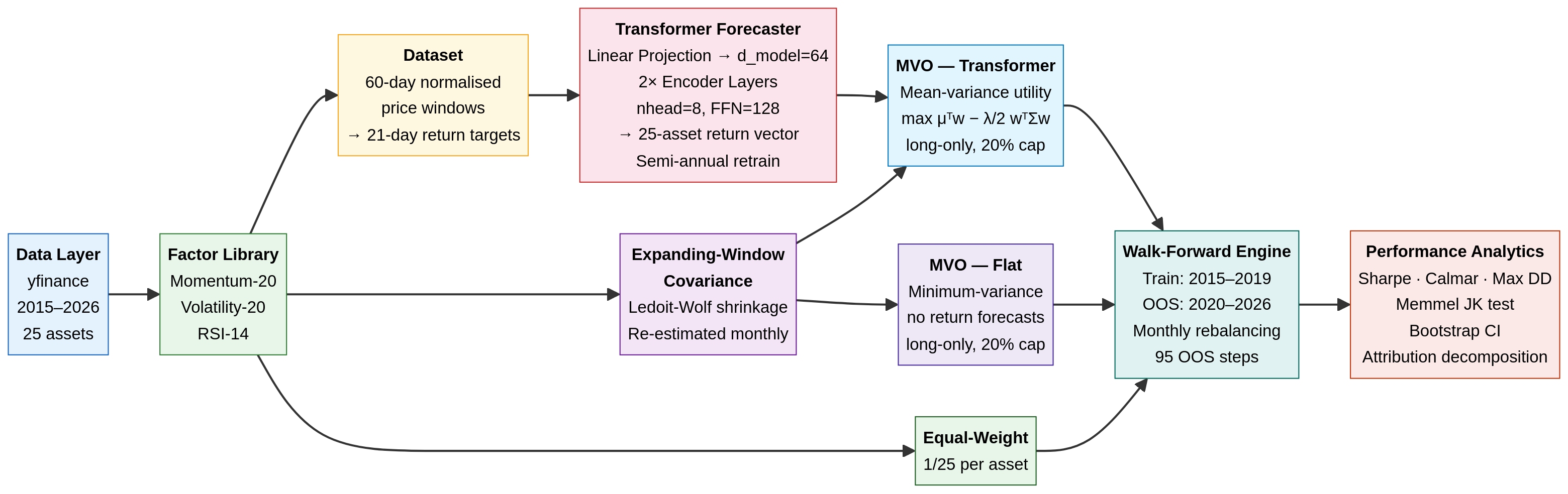
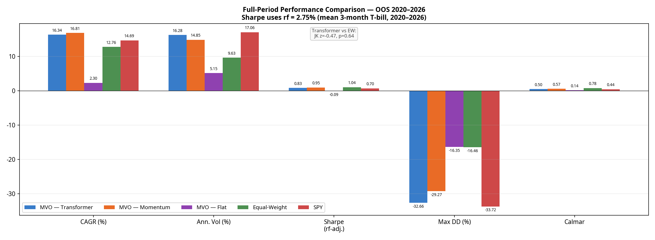
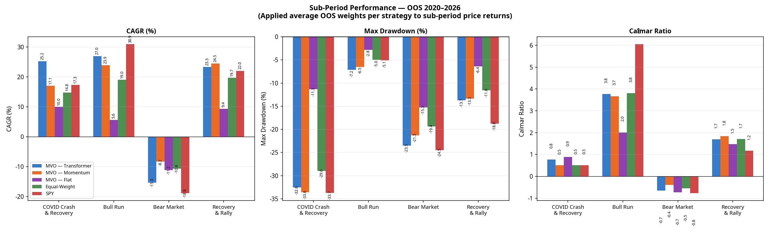
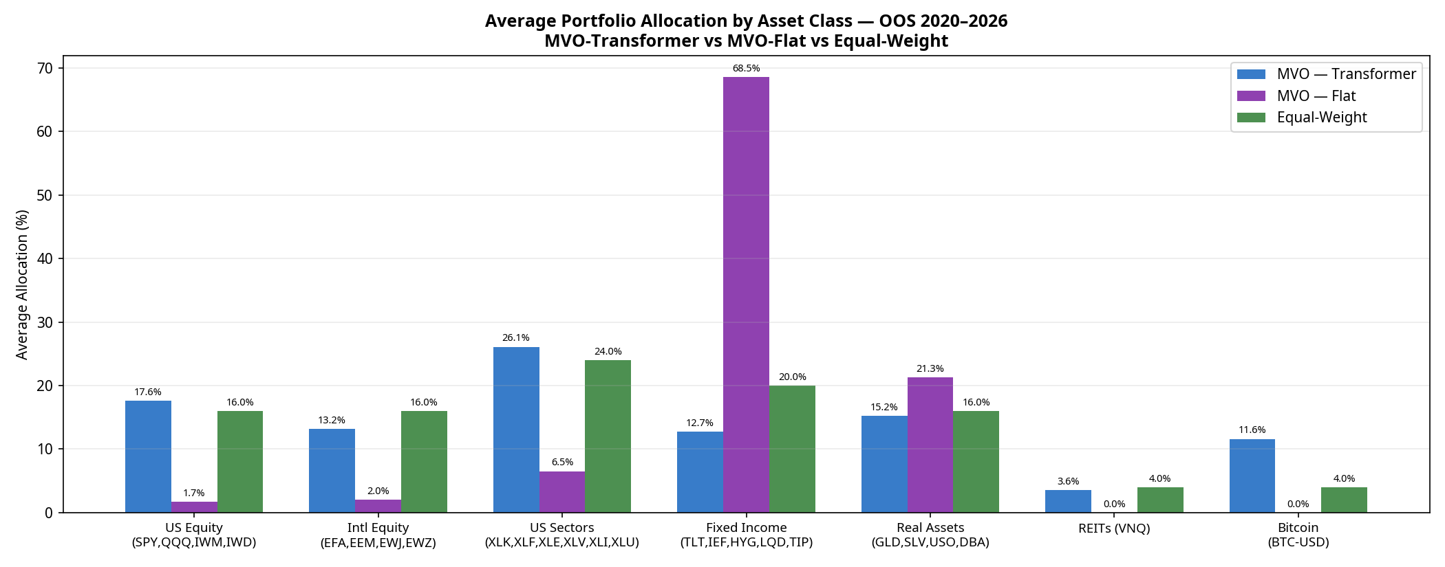
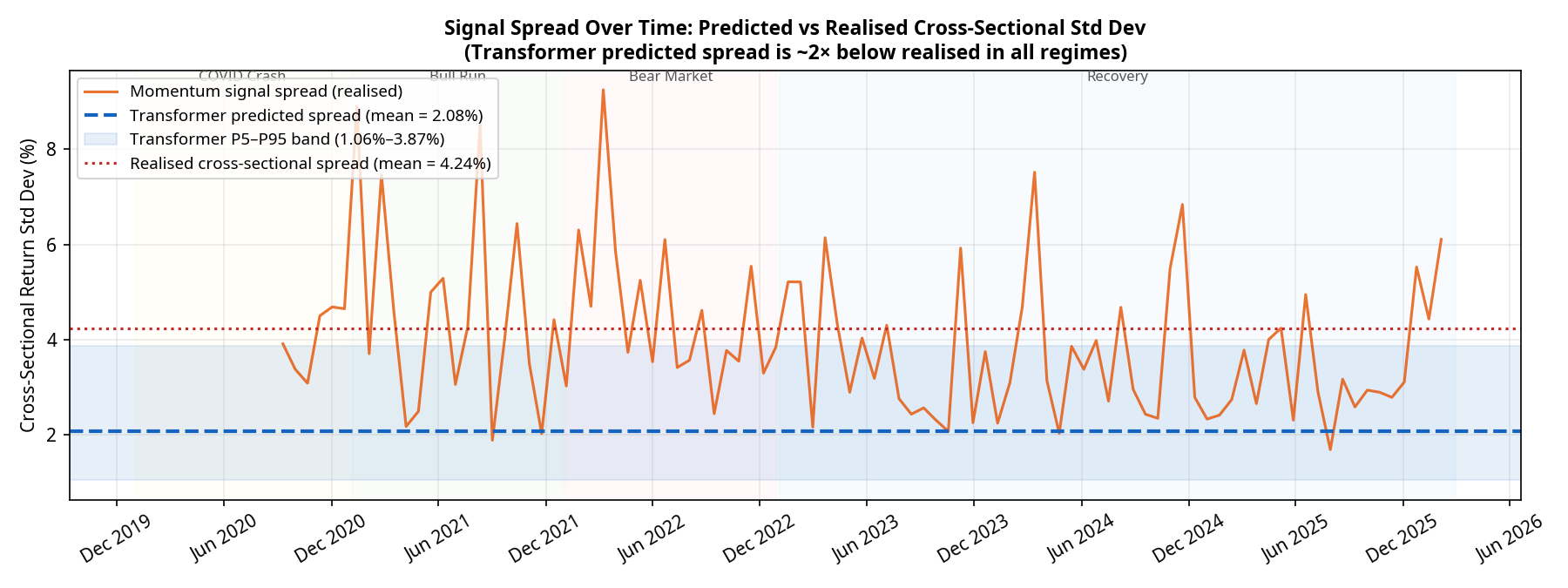

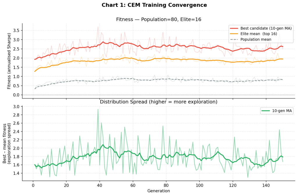
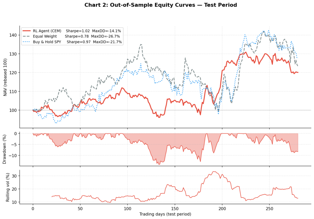
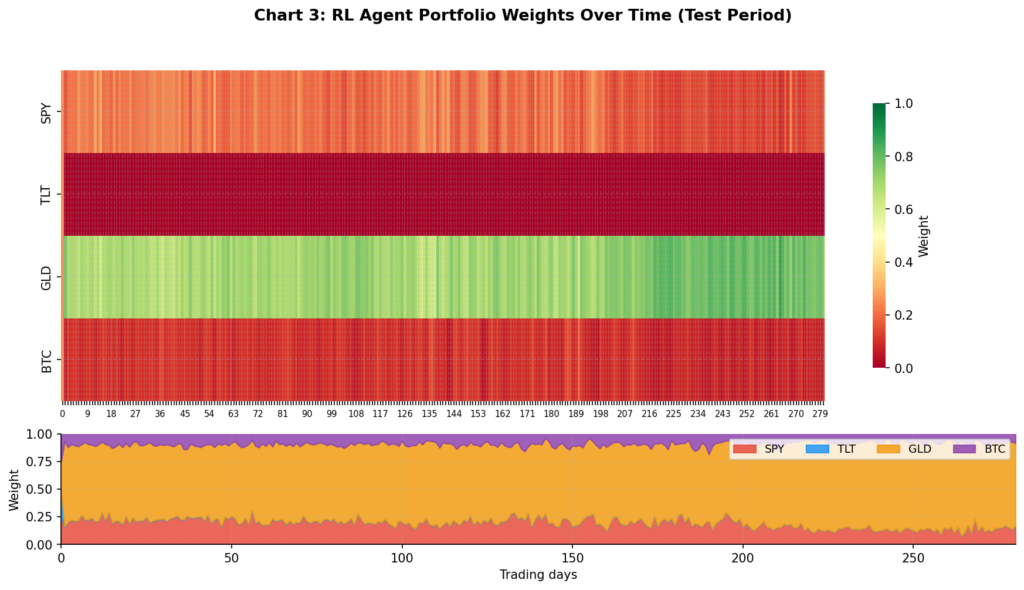
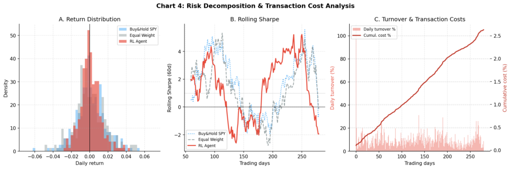

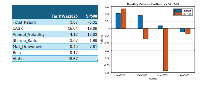
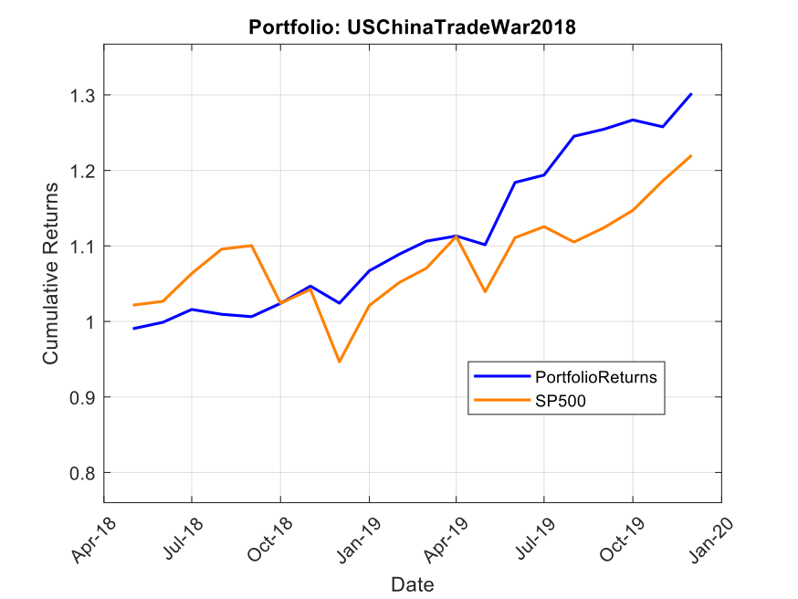
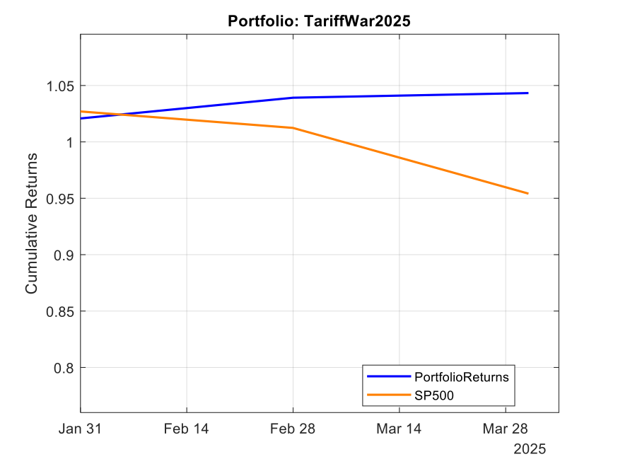


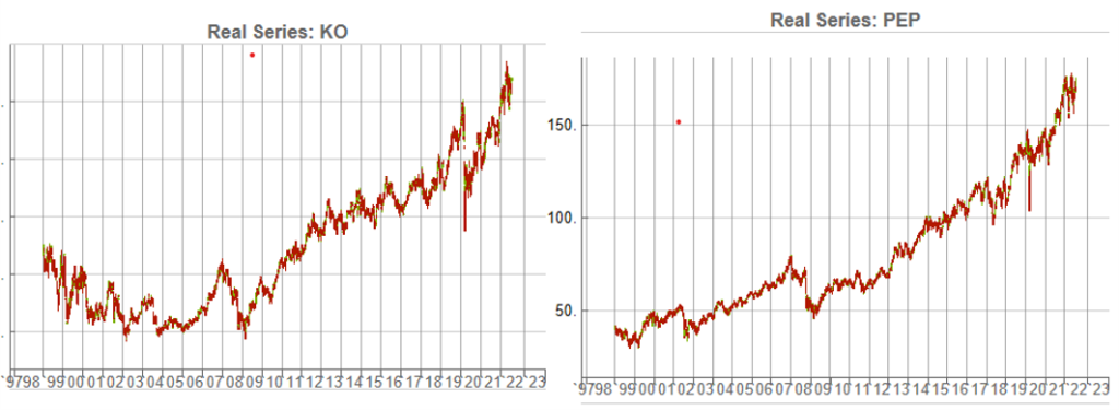
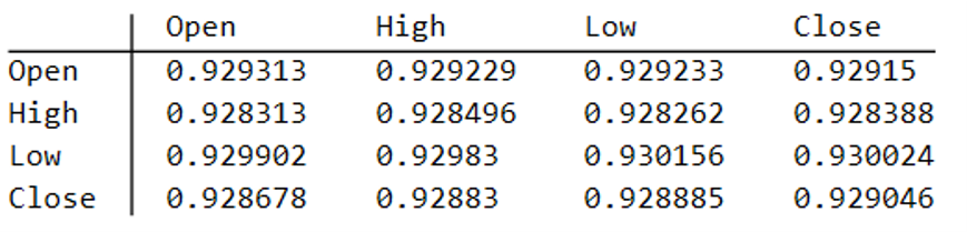
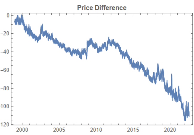
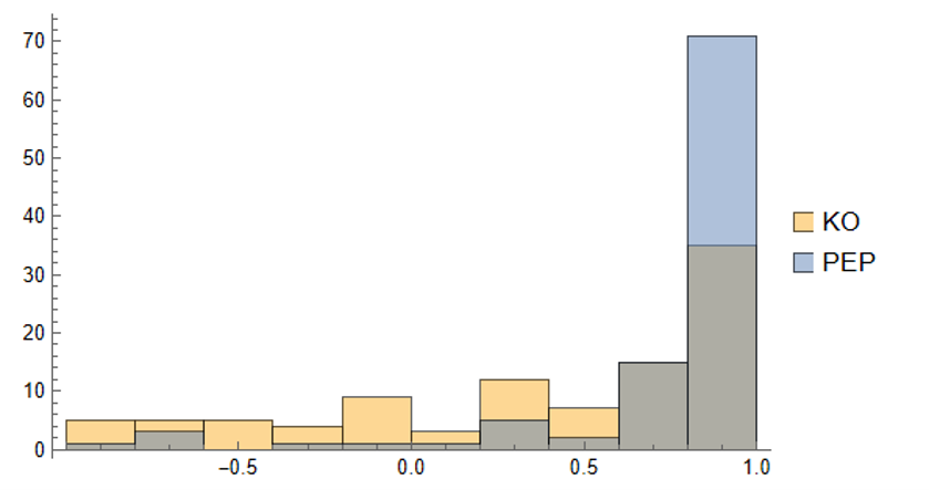
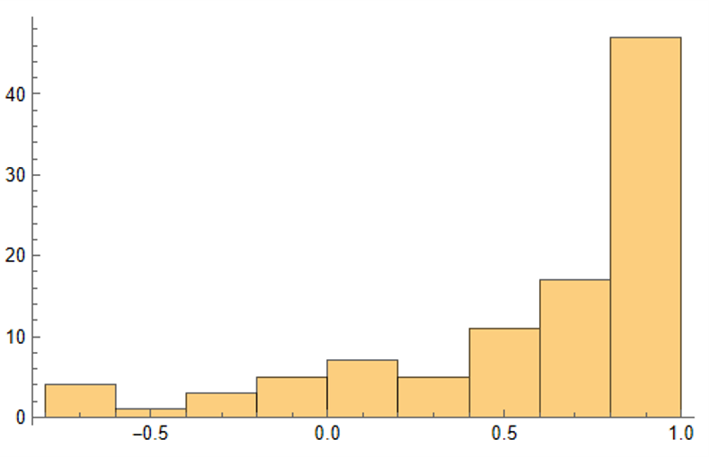
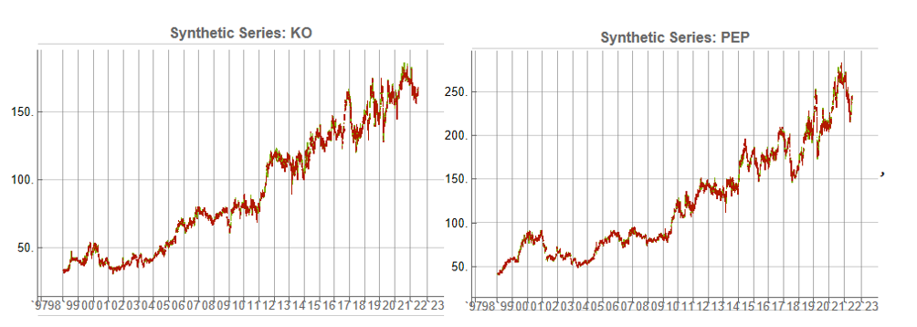
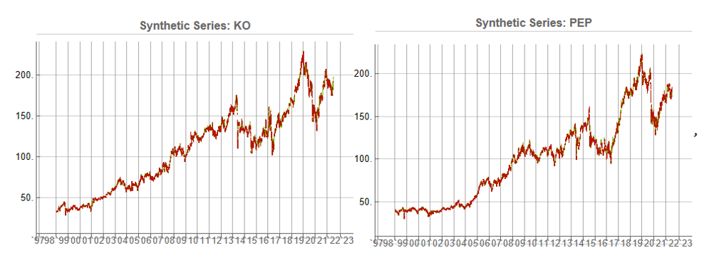
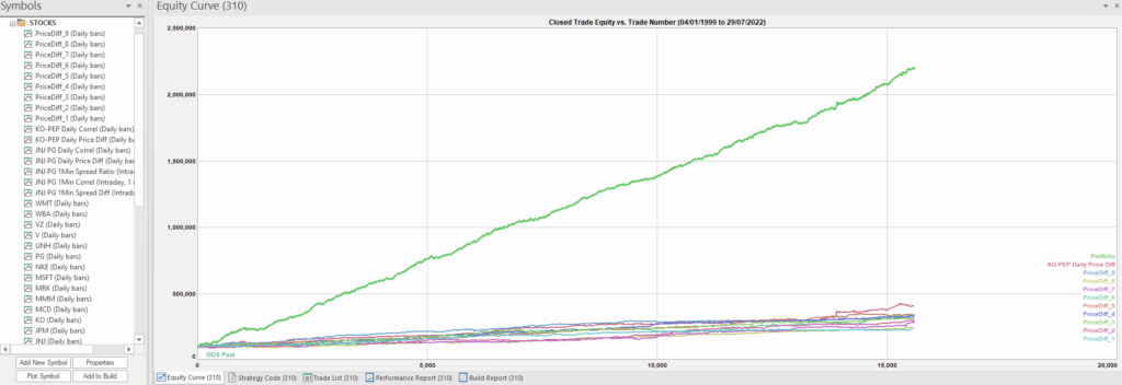
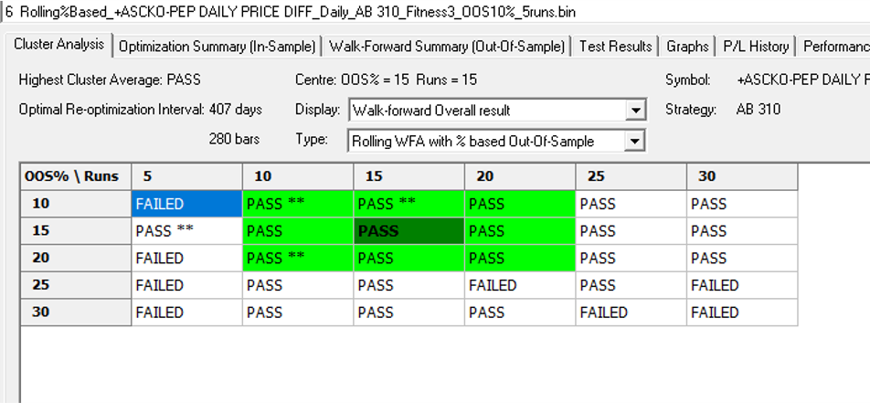
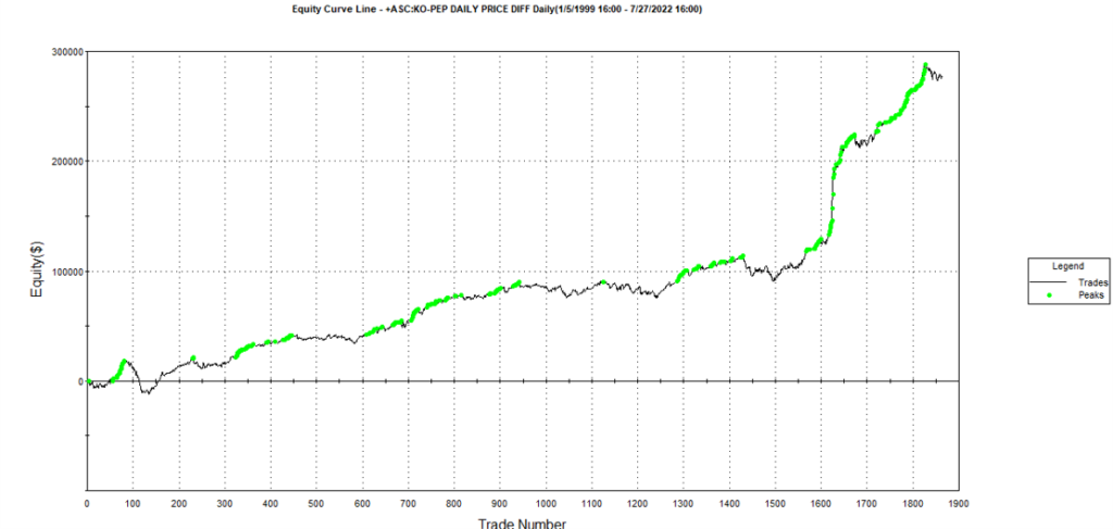
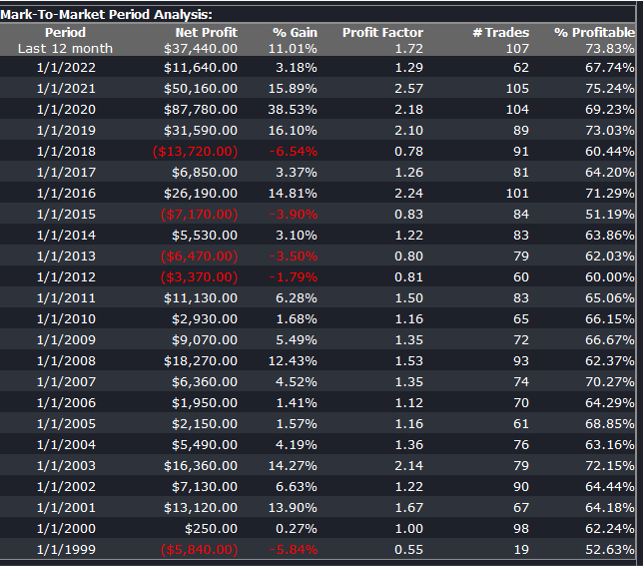


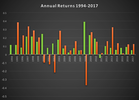

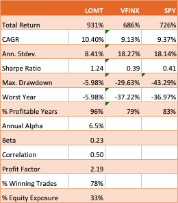
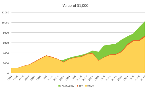
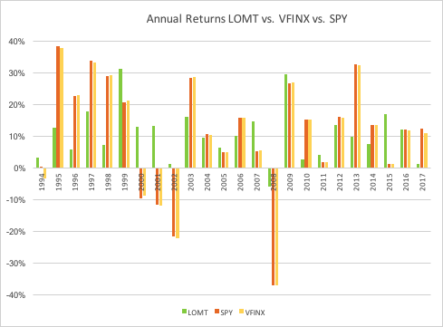


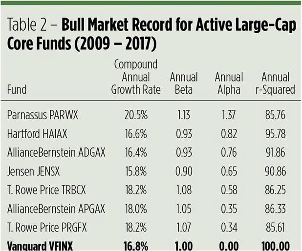


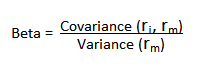
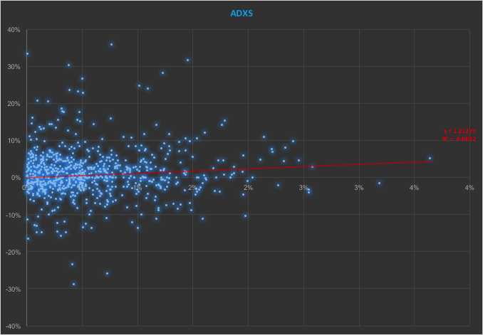
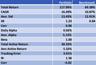
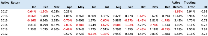
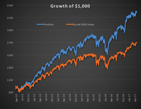
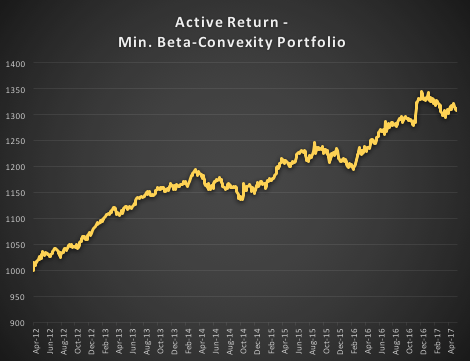


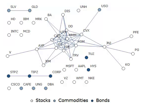

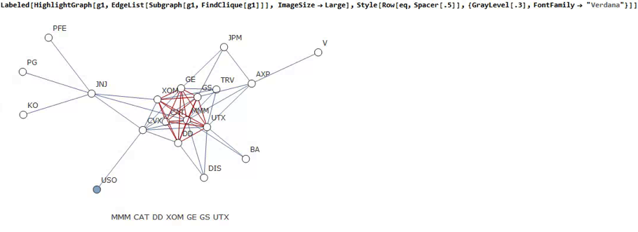
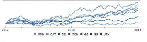
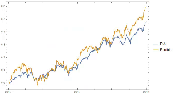
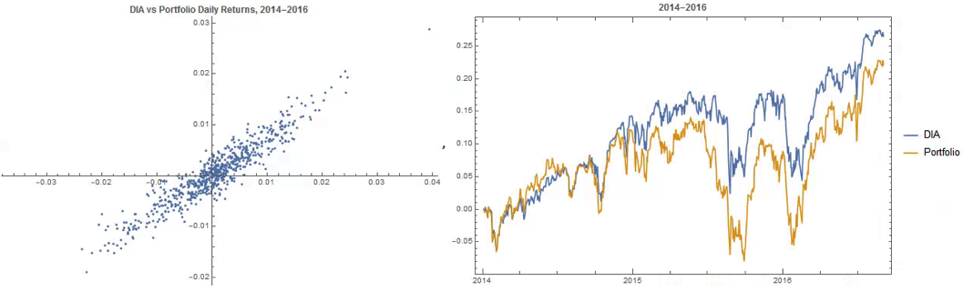

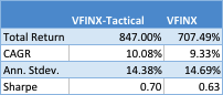