I want to take a look at a trading strategy in the GDX Gold ETF that has attracted quite a lot of attention, stemming from Jay Kaeppel’s article: The Greatest Gold Stock System You’ll Probably Never Use .
The essence of the approach is that GDX has reliably tended to trade off during the day session, after making gains in the overnight session. One possible explanation for the phenomenon is offer by Adrian Douglas in his article Gold Market is not “Fixed”, it’s Rigged in which he takes issue with the London Fixing mechanism used to set the daily price of gold
In any event there has been a long-term opportunity to exploit what appears to be a market inefficiency using an extremely simple trading rule, as described by Oddmund Grotte (see http://www.quantifiedstrategies.com/the-greatest-gold-stock-system-you-should-trade/):
1) If GDX rises from the open to the close more than 0.1%, buy on the close and exit on the opening next day.
2) If GDX rises from the open to the close more than 0.1% the day before, sell short on the opening and exit on the close (you have to both sell your position from number 1 but also short some more).

Unfortunately this simple strategy has recently begun to fail, producing (substantial) negative returns since June 2013. So I have been experimenting with a number of closely-related strategies and have created a simple Excel workbook to evaluate them. First, a little notation:
RCO = Return from prior close to market open
ROC = return from open to close
RCC = Return from close to close
I also use the suffix “m1” to denote the prior period’s return. So, for example, ROCm1 is yesterday’s return, measured from open to close. And I use the slash symbol “/” to denote dependency. So, for instance, RCO/ROCm1 means the return from today’s open to close, given the return from open to close yesterday.
In the accompanying workbook I look at several possible, closely related trading rules, and evaluate their performance over time. The basic daily data spans the period from May 2006 to July 2013 and in shown in columns A-H of the workbook. Columns I-K show the daily RCO, ROC and RCC returns. The returns for three different strategies are shown in columns L, N and P, and the cumulative returns for each are shown in columns M, N and Q, respectively.
The trading rules for each of the strategies are as follows:
COL L: RCO/ROCm1>0.5%. Which means: buy GDX at the close if the intra-day return from open to close exceeds 0.5%, and hold overnight until the following morning.
COL N: ROC/ROCm1>1%. Which means: sell GDX at today’s open if the intra-day return from open to close on the preceding day exceeds 1% and buy at today’s close.
COL P: ROC/RCCm1>1%. Which means: sell GDX at today’s open if the return from close to close on the preceding day exceeds 1% and buy at today’s close.
COL R shows returns from a blended strategy which combines the returns from the strategies in columns N and P on Mondays, Tuesdays and Thursdays only (i.e. assuming no trading on Wednesdays or Fridays). The cumulative returns from this hybrid strategy are shown in column S.
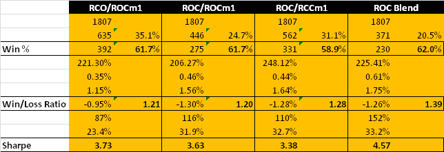
We can now present the results from the four strategies, over the 7 year period from May 2006 to July 2013, as shown in the chart and table below. On their face, the results are impressive: all four strategies have Sharpe ratios in excess of 3, with the blended strategy having a Sharpe of 4.57, while the daily win rates average around 60%.

How well do these strategies hold up over time? You can monitor their performance as you move through time by clicking on the scrollbar control in COL U of the workbook. As you do so, the start date of the strategies is rolled forward, and the table of performance results is updated to include results from the new start date, ignoring any prior data.
As you can see, all of the strategies continue to perform well into the latter part of 2010. At that point, the performance of the first strategy begins to decline precipitously, although the remaining three strategies continue to do well. By mid-2012, the first strategy is showing negative performance, while the Sharpe ratios of the remaining strategies begin to decline. As we reach the end of Q1, 2013, only the Sharpe ratio of the ROC/RCCm1 strategy remains above 2 for the period Apr 2013 to July 2013.
The conclusion appears to be that there is evidence for the possibility of generating abnormal returns in GDX lasting well into the current decade. However these have declined considerably in recent years, to a point where the effects are likely no longer important.