September 2026
I gave a research agent four years of prices with no predictable structure in them — none, by construction — and it came back with a long/short book, an in-sample Sharpe of 2.1, and a paragraph explaining the economics of an effect that does not exist.
That is the measurement in this post. The more useful result is the second one: 88% of that number is accounted for by two integers — how many backtests the agent ran, and how many of the winners it blended into the book it reported. Only one of those is in the log everybody proposes to collect.
This closes a sequence. In August, having built an agentic research pipeline in May and measured a 2× lift in hypotheses tested per week, I priced a risk I had not thought to price: independent research runs against the same model produce books correlated at 0.62, a crowding exposure that appears in nobody’s risk report. That post ended with a claim I stated and did not measure — that faster hypothesis generation makes overfitting worse rather than better. This is the measurement, and my pre-registered prediction about how it would come out was wrong.
The one property agentic research has that human research never had
Every multiple-testing correction in finance founders on the same rock: you cannot observe the denominator. Harvey, Liu and Zhu built their t-statistic hurdle on an estimate of how many factors had been tried across the profession, not how many were published [1]. Harvey’s 2017 AFA presidential address is largely an argument about unreported trials [2]. The Deflated Sharpe Ratio requires you to supply the number of trials, and its authors are candid that in practice you are guessing [3]. Each method asks the researcher a question the researcher cannot honestly answer: how many things did you try before this one?
An agentic pipeline is different in exactly one respect. It has to ask the harness for every backtest it runs. The trial count is not a memory or an act of professional honesty. It is a log file.
So I built a minimal research agent, gave it one tool, recorded everything, and checked what the log is worth. The short answer is that it is worth less than I expected, for a reason that turns out to be measurable and fixable.
Setup
The harness. One command: submit up to 25 expressions, receive their in-sample scores. At most 12 such calls. The agent never sees prices, dates, tickers, or the holdout — the panel is anonymised to integer asset IDs and an integer time index, and the holdout files were physically absent from the filesystem while the runs executed. Every submission is logged with a timestamp, alongside a one-line hypothesis per batch and a free-text journal. The run ends when the agent reports exactly three signals.
What a “book” is, and the two counts that matter. Every arm’s output is scored the same way: three signals, equal-weighted into one book. The pre-registered primary rule takes the three highest-scoring signals a run evaluated, not the three it chose to report — the gap between the two is small and is itself reported below. N is the number of trials in the log. k is the number of additive legs in the resulting book: three for a searcher whose signals are single expressions, more for one whose signals are themselves sums. Those two integers carry the whole argument.
The signal language. A small price-only grammar: returns, moving averages, rolling moments, range position, rolling beta and correlation to the equal-weight panel, plus cross-sectional and time-series normalisations and arithmetic. It is the grammar from the August post, which matters — it was fixed before this hypothesis existed. Each signal becomes a dollar-neutral, rank-weighted long/short book with a one-day implementation lag.
The comparison arms. Three mechanical arms plus a no-selection placebo. The two that search run at the agent’s interaction schedule — 12 rounds of 25 candidates, feedback once per round. Matching rounds rather than evaluations is deliberate: in adaptive data analysis the damage scales with how many times you look and act, not with the raw query count [4].
| Arm | What it is |
|---|---|
| AGENT | The LLM researcher above |
| OPT | Evolutionary search over the same grammar, at three selection pressures (soft, medium, hard — how aggressively each generation is bred from the current leaders) |
| CANON-SAMPLER | Canon-shaped expressions with jittered parameters, no feedback — prior direction without optimisation |
| CANON placebo | Twelve published anomalies in the same grammar, no selection at all |
The data. The primary setting is synthetic: factor-structured panels with regime-switching volatility and fat tails, and zero predictability by construction. Volatility is forecastable; returns are not. The true Sharpe of every signal is zero, so every point of in-sample Sharpe is selection, and I can generate independent panels at will. The second setting is the real NASDAQ panel from the August post — 1,280 names, 2018–2023, train through 2021, holdout 2022 to May 2023.
The analysis plan, estimators, inclusion rule and predictions were committed to git before the first agent run. The repo holds the commit history, every harness log with its batch notes and research journals, a manifest of all 227 attempted runs including the five abandoned and why, and a list of every deviation from the plan.
1. What a research agent does with data that contains nothing
Twelve independent zero-alpha panels, one agent run each, identical prompt to the real-panel runs.
Every run found something. Every run wrote a confident rationale. From the report of a run on a panel whose returns are serially unpredictable by construction:
“All three combine the two independently validated engines: long-horizon cross-sectional mean reversion (ma 120-250, plateau confirmed across ret, ma, minr and maxr formulations at horizons 60-250) and a weekly return echo (returns from days t-8 to t-5 predict positively, with a coherent oscillating lag profile).”
There is no echo. There is no reversal. There is nothing.
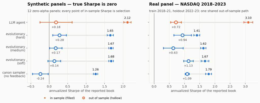
| Zero-alpha panels | Reported in-sample Sharpe | Realised out-of-sample Sharpe |
|---|---|---|
| LLM agent (12 runs) | 2.12 (SE 0.10) | +0.18 (SE 0.44) |
| Evolutionary, soft (12 panels) | 1.68 (SE 0.07) | +0.14 (SE 0.24) |
| Evolutionary, medium | 1.67 (SE 0.05) | +0.17 (SE 0.22) |
| Evolutionary, hard | 1.65 (SE 0.11) | +0.28 (SE 0.22) |
| Canon sampler, no feedback | 1.26 (SE 0.08) | −0.24 (SE 0.29) |
The reported book is the equal-weight composite of the three highest-scoring signals a run evaluated — the pre-registered primary rule, which is why it differs slightly from what the agent chose to report. True out-of-sample Sharpe is zero for every arm by construction, and every row is consistent with that. Standard errors are across panels.
A Sharpe ratio of 2.12, in-sample, on a book, over four years of daily data, from a panel with no signal in it.
A little over half of that is textbook. The expected maximum Sharpe of a single expression over the agent’s own median 146 logged trials is 1.15 (SE 0.03, across the twelve panels’ random-expression pools) — the expected-maximum-Sharpe effect [3], computed here as the exact order statistic over an empirical null pool drawn from the same grammar. That accounts for 54% of the 2.12. Note what the benchmark cannot do: those are single expressions, and it takes a single expression as the answer. Hold that thought — the missing 0.97 is the subject of section 3.
The agent’s own judgment is not the problem. It usually declines to report its top three by raw score, preferring what it calls “plateau” specifications; that restraint moves the number by 0.03 (2.08 chosen versus 2.12 argmax).
2. It manufactures more than a machine built to overfit
Paired by panel, against the evolutionary optimiser at the identical interaction schedule, using only the twelve primary runs:
| Contrast, in-sample Sharpe (12 paired panels) | Difference | SE | t |
|---|---|---|---|
| Agent − evolutionary (soft) | +0.44 | 0.11 | +3.9 |
| Agent − evolutionary (medium) | +0.45 | 0.11 | +4.1 |
| Agent − evolutionary (hard) | +0.46 | 0.09 | +5.2 |
On the real panel the gap is larger: 3.10 against 1.41–1.67.
That is the in-sample difference, and it is solid. The out-of-sample differences are not: those contrasts carry standard errors of 0.35 to 0.42, against a minimum detectable effect of about 1.0 Sharpe, and the pre-registered block bootstrap on the real panel returns a 95% interval of [−0.53, +1.99] for the agent’s realised Sharpe alone. Nothing in this study establishes that the agent’s books perform worse out of sample than a mechanical optimiser’s. What it establishes is that at a matched interaction budget, the agent converts noise into reported Sharpe more efficiently.
My pre-registered prediction was the opposite — that the model’s priors would act as a regulariser, keeping it in the published canon rather than in the noise, so it would overfit less. Wrong, at t ≈ 4.
3. Where the extra Sharpe comes from is not more searching
The mechanism is in the logs, and it is not model priors.
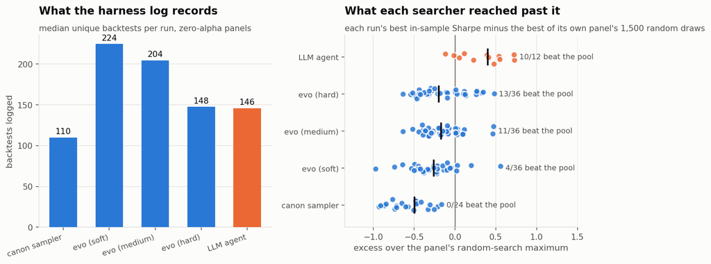
The agent logs a median of 146 unique backtests per zero-alpha run, against 148–225 for the evolutionary arms: level with the hardest setting, well below the softer ones. It is not searching harder — and note that the largest gap in the table above, +0.46, is against the arm that runs the same number of trials.
The difference is in what gets reported. Every run reports three signals, which are equal-weighted into one book. For the mechanical arms each of those three is a single expression, so the book has 3 legs. The agent’s three are themselves sums: a median of 4.2 legs each on zero-alpha panels, so its book carries about 12.5. That is the second integer, and no trial-count correction records it.
To isolate it I ran a controlled experiment on the zero-alpha panels with no agent involved: draw N random expressions, keep the top k by in-sample Sharpe, equal-weight them into a book, and record what the book reports.
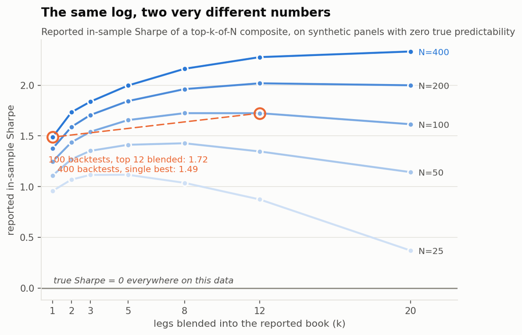
Moving between curves is the familiar overfitting-versus-trials axis. Moving right along a curve is the aggregation axis nobody logs. The two trade off against each other: a pipeline that logs 100 backtests and blends its top 12 reports 1.72, while one that logs 400 and reports a single best reports 1.49. No alpha in either case, and the first pipeline’s log looks four times cleaner.
The arithmetic is standard portfolio algebra pointed at noise. Selecting k signals on in-sample performance and averaging them keeps the selected mean and cuts the variance — but the legs are not independent, so the gain is √(k / (1 + (k−1)ρ̄)), not √k. Fitting that form column by column over the monotone region gives ρ̄ of 0.41–0.47 at the trial counts that matter here, a ceiling of about 1.5× however many legs you add. That is why the curves flatten. They turn down at small N for a different reason: once k is a large fraction of N you are averaging in candidates that were barely selected at all. Novy-Marx made the combination point for strategies built from multiple signals and derived corrected critical values for it [5]; what is new here is an agent that was never asked to combine anything doing it unprompted, and the interchangeability of the two axes at a fixed log.
The closure. Take each run’s own logged trial count and its own book leg count, look up what blind top-k-of-N selection produces at that point on the surface, and compare:
| Arm | Median trials | Legs in book | Blind top-k-of-N predicts | Actually reported | Residual |
|---|---|---|---|---|---|
| LLM agent | 146 | 12.5 | 1.86 | 2.12 | +0.26 |
| Evolutionary, hard | 148 | 3 | 1.68 | 1.65 | −0.03 |
| Evolutionary, medium | 205 | 3 | 1.73 | 1.67 | −0.05 |
| Evolutionary, soft | 225 | 3 | 1.77 | 1.68 | −0.09 |
| Canon sampler | 110 | 3 | 1.56 | 1.26 | −0.31 |
Two integers and no model price the evolutionary arms to within 0.09, and account for 88% of the agent’s number. The residual is +0.26 (t ≈ 2.1 once the surface’s own estimation error is propagated) — small next to the 1.86 that blind selection explains. And the leg axis alone carries most of the agent’s edge over the mechanical searchers: holding trials at the agent’s own 146 and moving the book from 3 legs to 12.5 adds +0.25, against a measured agent-minus-mechanical gap of +0.45.
So the agent beats the optimiser and is beaten by blind selection at its own operating point, and both facts have one cause. It blends; they do not.
That also settles what happened to the estimator I pre-registered. I had planned to report an effective trial count — the random draws from this grammar needed to match a run’s best score. It cannot be computed for most agent runs: 10 of 12 exceed the best their own panel’s 1,500-draw random pool reached, so no trial count reproduces them. That is partly a property of a finite pool and it is not agent-specific — 13 of 36 hard evolutionary runs also clear their pool — so nothing here rests on it. The direction is informative, though: a deeper random-expression pool (depth 6, mean complexity 5.9 against the shallow pool’s 3.6) lifts the 99th percentile from 0.95 to 1.24 and the maximum to 1.79 without closing the gap, because random expressions almost never build composites — mean legs 1.15.
Depth is not the axis. Blending is.
4. The real panel
Six agent runs on the NASDAQ panel, trained through 2021, scored on 2022 to May 2023.
| Real panel | Train | Holdout | Legs in book | Daily turnover |
|---|---|---|---|---|
| LLM agent (6) | 3.10 (SE 0.15) | +0.72 (SE 0.18) | 6.0 | 0.24 |
| Canon sampler (5) | 1.79 (SE 0.10) | +1.09 (SE 0.07) | 3 | 0.45 |
| Evolutionary, soft (5) | 1.67 (SE 0.13) | +1.13 (SE 0.16) | 3 | 0.43 |
| Evolutionary, medium (5) | 1.62 (SE 0.09) | +0.63 (SE 0.32) | 3 | 0.26 |
| Evolutionary, hard (5) | 1.41 (SE 0.10) | +0.94 (SE 0.29) | 3 | 0.49 |
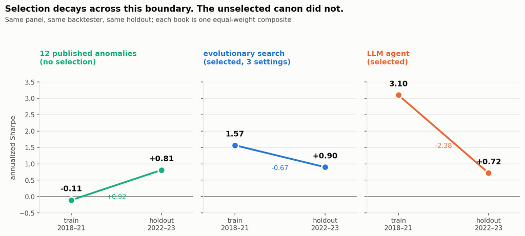
| 12 published anomalies, no selection | −0.11 | +0.81 | — | 0.14 |
The last row is the control that makes the rest interpretable, and it is scored exactly like every other row — one equal-weight composite, same backtester, same holdout — with no selection applied. It does not decay across this boundary. It improves, from −0.11 to +0.81. The 2022–23 environment was kinder to these exposures on this universe than the training window was.
So the regime component of the agent’s decay is not merely small; it is negative. The control licenses one claim and not a stronger one: the unselected canon did not decay here, so the regime cannot explain the agent’s 2.4-point gap. It does not follow that selection explains all of it — the canon composite is loaded the opposite way from a book selected to score 3.10 in the training window, and the pre-registered random-search leg that would have measured the selection component directly was not run.
Note what the ordering does not do. It is not monotone — the medium evolutionary arm has the lowest holdout Sharpe of any arm, below the agent’s — and every one of those holdout differences sits inside the block-bootstrap intervals. The real panel cannot adjudicate between these arms.
Turnover does not explain the gap either: the agent’s books turn over 24% of gross per day, at the low end of the arms rather than the high end.
5. What the number is worth, and what it is not
The obvious next move is to use the zero-alpha number as a correction: subtract what the pipeline manufactures from noise off the face value of what it reports on real data. Since true Sharpe on the synthetic panels is zero by construction, the manufactured component is the reported in-sample Sharpe itself — 2.12 for the agent. That gives 3.10 − 2.12 = 0.98 predicted against 0.72 realised, which looks like a hit.
It is not. Run the same arithmetic for every arm:
| Arm | Zero-alpha manufacture | Real face | Predicted | Realised | Predicted − realised |
|---|---|---|---|---|---|
| LLM agent | 2.12 | 3.10 | 0.98 | 0.72 | +0.26 |
| Evolutionary, soft | 1.68 | 1.67 | −0.00 | 1.13 | −1.13 |
| Evolutionary, medium | 1.67 | 1.62 | −0.05 | 0.63 | −0.68 |
| Evolutionary, hard | 1.65 | 1.41 | −0.25 | 0.94 | −1.18 |
| Canon sampler | 1.26 | 1.79 | 0.54 | 1.09 | −0.55 |
A negative last column means the haircut left too little on the table. Mean error −0.66. The correction under-predicts realised performance in four arms out of five, and the agent’s near-miss is the one that landed the other way. These are five books on one shared holdout path, not five independent draws, so this is one observation with five views of it rather than five tests. The reason is in the previous table: this holdout carried a tailwind of roughly +0.9 for canonical exposures, which a calibration built on noise cannot know about.
So the zero-alpha number measures how much in-sample Sharpe your pipeline manufactures from nothing. It is not a forecast of out-of-sample performance, because realised performance also contains whatever the regime does to your exposures, and that term is not small. What it is worth is the overstatement:
| Selection overstatement — $100M book at 10% target volatility | |
|---|---|
| Face in-sample Sharpe of the reported book | 3.1 |
| Measured manufacturing capacity (zero-alpha calibration) | 2.1 |
| Annual return overstatement | ≈ $21M |
| In basis points of notional | ≈ 2,100 bp |
The amount by which the in-sample report overstates, measured on data containing no alpha. Gross of costs, rounded. Not a forecast and not strategy P&L: the row above shows the haircut does not predict realised returns. Absolute performance levels on a survivorship-conditioned panel are not defensible and no such claim is made.
Things that did not work
Two pre-registered predictions failed. The first, above: the prior did not act as a regulariser. The second concerned the planted-alpha panels, where I buried two effects of equal calibrated in-sample strength — one canon-shaped (short-horizon reversal), one deliberately anti-canon (a kurtosis effect the literature points away from) — expecting the agent to find the canon-shaped one better and the mechanical arms to show no such asymmetry. Both halves were wrong. At the higher plant strength the agent captured the anti-canon plant better (0.50 versus 0.41), and it was the evolutionary arm that showed the large asymmetry (0.87 versus −0.02) and delivered more of the real alpha out of sample (1.15 versus 0.50). The comparison is confounded — the plants were matched on in-sample strength, but their oracle holdout Sharpes came out at 0.46 and 1.30 — and the agent contributes four runs per cell.
A metric that dissolved against its null — for the second post running. Regressing the agent’s real-panel books on the twelve-anomaly basis gives a mean R² of 0.50: the agent is largely reproducing published anomalies. Run the same regression on random expressions from the same grammar and you get 0.72. Noise projects onto the canon basis better than the agent’s books do — so the metric ranks the agent as less canonical than random noise, which is not a statement about the agent at all. It measures the dimensionality of price-signal space. The lesson is cheap and general: any spanning statistic needs a null drawn from the same generator, or it is measuring the basis.
The look-ahead screen cannot fire. The holdout sits inside the model’s training corpus, so I pre-registered a one-sided screen against block-bootstrap continuations of the training panel — futures the model cannot have seen. Resampling training returns reproduces the structure the books were selected on, so the synthetic benchmark runs at 1.5–2.0 Sharpe for selected books and the statistic is negative by construction (Δ = −0.92; −1.64 under the demeaned variant). It found no evidence of pretraining leakage; it also could not have. The construction is in the repo.
The model changed underneath the experiment. Two-thirds of the way through, a rate limit forced a checkpoint switch. Four partly-completed runs were abandoned under the pre-registered inclusion rule and re-run on the same four panels; a fifth run was abandoned after I contaminated it with an operator timing probe. All five are in the manifest. The twelve primary zero-alpha runs are all on the first checkpoint. Three bridge runs on the second checkpoint over the same panels reported 2.74 against 2.09 for the first checkpoint on those panels. That gap is not identified, by this post’s own mechanism: the bridge runs used their full 300-trial budget against the primary runs’ ~145, and at fixed leg count the surface predicts about half of the 0.65 gap from trials alone. Three runs is an anecdote in any case; it is reported because it is the clearest available evidence that these numbers are a snapshot of specific checkpoints. Which checkpoint served each run was never recorded — it is reconstructed from run identifiers and timing, which is a defect in my instrumentation and is flagged in the repo.
What this does and does not show
It does not show that agent-generated books underperform mechanically-generated ones out of sample. Those contrasts are inside their standard errors and the design cannot resolve them.
It does not show that a zero-alpha haircut predicts realised performance. Section 5 shows it does not.
The limitations that matter, in order. This is a minimal single-loop researcher — one agent, one tool, ≤300 trials, no holdout gate, no research committee — one to two orders below a production pipeline, and everything a real stack adds either raises the trial count or is a control whose value this same instrumentation would demonstrate. It is a floor. One model family, and a checkpoint that changed mid-study; the cross-family experiment could not be run. The real panel is one shared out-of-sample path on a survivorship-conditioned universe inside the model’s training corpus, so every real-panel number here is descriptive and the inference lives in the synthetic arm. Twelve panels is a small cross-section and every interval is wide. And the mechanical arms are matched on rounds and grammar but not perfectly: the evolutionary arm is seeded and mutated at bounded expression depth while the agent writes free-form strings, so the agent searches a strictly larger subspace — which is consistent with the finding, since composite depth is exactly the axis that matters, but it means “same grammar” is doing less work than it sounds like.
Eleven deviations from the pre-registration — the censored trial-count estimator, the random-search decomposition leg that was not run, 60 continuations instead of 200, the warm-start evaluation basis, a prompt revised after the plan was committed, and the rest — are listed in DEVIATIONS.md.
So what do you do
Build the surface for your own stack. This is the differentiated move and it costs almost nothing. Construct a panel matched to your universe — same factor covariance, same volatility dynamics, same fat tails — with the conditional mean stripped out, and verify the construction by checking that an oracle signal earns zero. Then run your own pipeline against it, unmodified, and record what it reports at each (trials, legs) pair you actually operate at. That grid is your pipeline’s manufacturing capacity in the units you use, and you can look up any future result on it. For the pipeline here it was 2.1 Sharpe. The generator and the surface code are in the repo and the whole thing runs on a laptop.
Log two numbers, not one. The trial count is now an artifact rather than a memory, and a pipeline that cannot produce one is worse off than this toy. But on its own it prices nothing: a 12-leg book from 100 trials carries more selection than a single expression from 400, and only the first of those facts is in the log everyone proposes to keep. With both numbers you can look the answer up on your own surface. With one you cannot.
Then subtract, and stop there. The result tells you how much of the reported number is manufacturing. It does not tell you what the book will earn, because that also depends on what the regime does to your exposures — and section 5 shows that term is larger than the correction.
Every zero-alpha run in this study produced a good economic story — volatility term structure, lottery preference, reversal at horizons where reversal is documented — attached to nothing. The pipeline is a fine instrument. It is also, on data containing nothing, a machine for producing a Sharpe of 2.1 and a paragraph about why.
Code and data
Repo: jkinlay/agent-selection-surface
The repository contains the pre-registered analysis plan committed before the first run, a deviations list, the frozen prompt, the harness, the mechanical arms, the synthetic generator with its calibration constants, every run log with its batch notes and research journals, the manifest of all 227 attempted runs with dispositions and reasons, the backtester canary tests, and the analysis and figure code. Everything downstream of the LLM calls reproduces from seeds; the LLM calls are not re-runnable, which is why the logs are included in full.
Two requests of anyone re-running it. Run the zero-alpha arm first — it is what makes every subsequent number interpretable. And log the leg count, not just the trial count.
References
[1] Harvey, Liu & Zhu, …and the Cross-Section of Expected Returns, Review of Financial Studies 29(1), 2016.
[2] Harvey, Presidential Address: The Scientific Outlook in Financial Economics, Journal of Finance 72(4), 2017.
[3] Bailey & López de Prado, The Deflated Sharpe Ratio, Journal of Portfolio Management 40(5), 2014; Bailey, Borwein, López de Prado & Zhu, Pseudo-Mathematics and Financial Charlatanism, Notices of the AMS 61(5), 2014, for the expected-maximum-Sharpe result used in section 1.
[4] Dwork, Feldman, Hardt, Pitassi, Reingold & Roth, The reusable holdout: Preserving validity in adaptive data analysis, Science 349(6248), 2015 — guarantees degrade with the number of adaptive rounds, which is why every arm here is matched on rounds rather than evaluations.
[5] Novy-Marx, Backtesting Strategies Based on Multiple Signals, NBER Working Paper 21329, 2015 — in-sample test statistics inflate with the number of combined signals, with corrected critical values. The aggregation axis in section 3 is this effect, arrived at by an agent that was not asked to combine anything.
[6] skfolio, load_nasdaq_dataset — daily adjusted closes, 1,455 NASDAQ constituents, 2018-01-02 to 2023-05-31, documented by its authors as a stale dataset not intended for investment or commercial use. Filtered here to 1,280 names with median price ≥ $5; SHA-256 of the source file is in the analysis plan.
[7] Canonical anomalies in the placebo: Jegadeesh & Titman (1993) with the Carhart (1997) 12-1 construction; Jegadeesh (1990); Ang, Hodrick, Xing & Zhang (2006); George & Hwang (2004); Frazzini & Pedersen (2014); Boyer, Mitton & Vorkink (2010); Moskowitz, Ooi & Pedersen (2012); Novy-Marx (2012). The twelfth, a 60-minus-120-day momentum-acceleration variant, is a construction of my own.
Disclosure: I run systematic strategies. Nothing here is a recommendation, and no strategy discussed is one I trade. These are diagnostic quantities from a methodological experiment on a stale public dataset, not a track record.