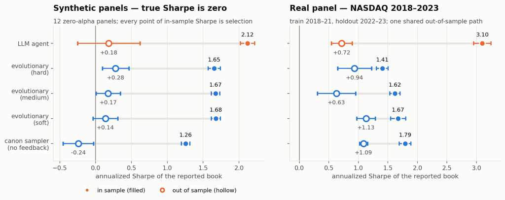

First, a correction
The panel in my September post was supposed to have zero alpha. It didn’t quite. The market factor carried a drift of 0.0002 per day and the betas were drawn N(1, 0.3), so a book that tilted towards high-beta names had a true Sharpe of about +0.22 on a panel I described as containing nothing. The generator also clipped daily returns asymmetrically, at [−0.5, +1.0], which leaves a name whose shock breaches the floor with a small positive mean that a book ranking on volatility can load on.
I found this while building the generator for this study, and priced both defects rather than describing them. Every one of the 294 books that post reported on its zero-alpha panels — both reporting rules, all five arms — has been re-scored on the published panel and on a twin that differs only in having the drift removed. The twin is bit-identical otherwise: the drift constant consumes no random draws, so the two panels share every innovation. The recomputation reproduces all 294 published Sharpe ratios to machine precision (maximum absolute error 8.9 × 10⁻¹⁶).
The clip is the smaller of the two, and separable the same way. Across the twelve September panels it binds on 7 of 6,000,000 daily returns — a daily return above +50% is not a common event in a panel of 2%-volatility names — and a volatility-ranked book collects +0.003 of out-of-sample Sharpe from it (SE 0.002, largest on any single panel 0.02). The rest of this section is the drift.
September’s headline is an in-sample number, and in sample the drift is worth almost nothing: the median drift component of in-sample Sharpe across all 294 books is +0.006, and for the agent’s own books it is −0.007, against a published 2.24. Out of sample the median by arm runs +0.004 to +0.019, and no arm-and-rule cell exceeds +0.025, against +0.27 for a book constructed deliberately to load on beta — a different measurement from the +0.22 above, which is that book’s absolute Sharpe on the September panels rather than its drift component. Individual books move more — the largest is +0.49 and the smallest −0.22, and book beta loadings run from −0.21 to +0.25 — so the drift is not invisible at the level of a single run. The pre-registered threshold I had set for retracting a September conclusion, a median drift component above 0.101, does not fire.
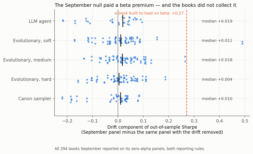
Every book September reported, on the published panel and on its drift-free twin
So September’s headline — that a research agent manufactures an in-sample Sharpe of 2.1 from nothing, and that 88% of it is explained by two integers in the log — stands. The generator does not. It has been replaced, the arithmetic is in the repository, and the correction is in this post rather than in a footnote, because a null you cannot verify is what this entire post is about.
Setup
The null. Factor-structured daily panels: 400 names, regime-switching volatility on the market and three latent factors, Student-t idiosyncratic shocks, lognormal dispersion in volatility. Zero drift, symmetric clipping, and — the part the September generator got wrong — separate random streams for structure (betas, loadings, volatilities, regime paths) and for innovations, so a fresh path can be drawn through the same world.
Verifying that a null is null is harder than writing one. The pre-registered acceptance test probed a constant-beta book and two oracle signals; it passed on two and, on the third, produced a +0.093 on the sixty study seeds that went away on a 120-seed replication. That episode is in the deviations file, and the acceptance file records the pre-registered failure rather than only the replication that passed. It also convinced me the test was too blunt, so there is a better one: 200 expressions drawn from the signal grammar before any panel existed, of which a median of 184 evaluate cleanly on a given panel, across 40 fresh null panels — 7,346 signal-panels, mean annualised Sharpe +0.017, 95% CI [−0.015, +0.048].
Two honest caveats on that. It is measured on the 1,000-day training window, not on the 2,000-day window the books are scored on. And on the exact sixty seeds this study ran, the residual tilt from the acceptance test is bounded at about +0.09 — larger than several of the out-of-sample numbers below. I flag them where they appear.
The pipeline being controlled. An evolutionary search over the same price-only grammar as the September post — returns, moving averages, rolling moments, range position, rolling beta and correlation, with cross-sectional and time-series normalisations. Twelve rounds of twenty-five expressions. The uncontrolled baseline reports the three highest in-sample Sharpes as an equal-weight book. Sixty seeds (9000–9059); 1,000 training days; 2,000 untouched days for scoring.
The two things worth measuring. Every control is placed on two axes.
How much manufactured Sharpe does it remove? Measured on panels with no alpha, and — this matters more than it sounds — measured on the number a user of that control would actually report. If a gate abstains, nothing is reported. If a control re-selects on a validation window, the researcher reports the validation-window number, not the training number they just threw away. If a control searches a shorter window, the researcher reports the shorter window’s Sharpe. Measuring every control on the original training window, which is what I did in the first pass of this study, flatters every re-selection control enormously and is the single largest correction here.
How much real alpha does it destroy? Measured on the same panels with a signal planted in them. Because each seed’s panels are drawn from identical innovations and differ only in the plant, the same book can be scored on both, which separates the exposure a noise-selected book has to the plant by construction from the gain that selecting on the planted panel actually adds. Only the second is “finding alpha”.
Two plants, and why. My first plant was calibrated to an in-sample Sharpe of about 1.0 — below the 1.77 the search manufactures from noise. A pipeline that ranks on in-sample Sharpe must then prefer the noise, so “the search fails to find real alpha” was a property of my calibration rather than a finding. There are now two, both calibrated on thirty seeds (8000–8029) rather than the three the first pass used: a weak plant and a strong one, with realised out-of-sample oracle Sharpes on the study seeds of 0.59 and 2.43.
The analysis plan, the predictions and the estimators were committed before the first search ran. Eighteen departures from them are logged, including several this study’s reviewers forced.
1. Selection manufactures the Sharpe. The search adds nothing.
Start with the uncontrolled pipeline on panels containing nothing:
| Uncontrolled pipeline, 60 null panels | Value |
|---|---|
| Reported in-sample Sharpe | 1.77 (SE 0.04) |
| Realised out-of-sample Sharpe, 2,000 days | +0.015 (SE 0.051) |
| One-way turnover, per day | 19.5% |
| Net of 5 bp per unit of turnover, at ≈2.5% book volatility | −1.00 |
Familiar enough. Now the part I did not expect. Take 200 expressions drawn at random from the grammar before any panel is generated — no search, no feedback, no breeding — and keep the best three by in-sample Sharpe. On the same kind of null panel that book has an annualised in-sample Sharpe of 1.99 (SE 0.05, 40 panels).
Put the evolutionary search on exactly the same footing — its own logged candidates, the same 700-day window, the same complete-case filter, top three re-selected on that window — and it reports 1.95 (SE 0.05, 60 panels). The difference is 0.04, Welch t = 0.60.
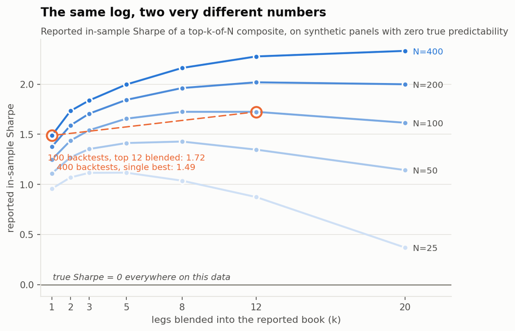
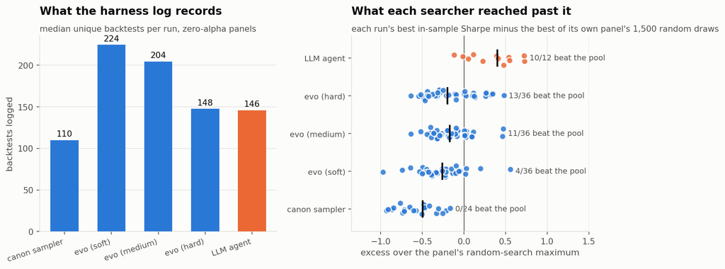
Twelve rounds of adaptive search, three hundred evaluations, mutation and crossover, and the machinery adds nothing measurable to the manufactured number. Picking three things out of a hundred and eighty-odd does all of the work. (The two arms run on different seed sets and are not paired; the pools are matched at 182 against 184 candidates after filtering, with participation ratios of 13 and 15.)
Whatever your research process is — an agent, a grid, a graduate student with a notebook — the quantity that produces the fictitious Sharpe is the size of the set you chose from, and nothing clever has to have happened inside.
2. The holdout that made the number bigger
Here is the reported in-sample Sharpe on panels with no alpha, for each control, measured on the window that control actually reports:
| Control | Reported Sharpe, null panels | Manufactured Sharpe removed | Abstains |
|---|---|---|---|
| Internal gate (search 750 days, pick on 250) | 3.08 | −0.74 | — |
| Internal gate + leg cap of 1 | 2.45 | −0.38 | — |
| 750-day search, no gate | 2.15 | −0.22 | — |
| Leg cap 12 | 1.78 | −0.01 | — |
| Uncontrolled baseline | 1.77 | — | — |
| Leg cap 1 | 1.65 | 0.07 | — |
| Budget 6 × 25 | 1.59 | 0.10 | — |
| Budget 12 × 12 | 1.56 | 0.12 | — |
| Budget 6 × 12 | 1.42 | 0.20 | — |
| Out-of-path gate (fresh innovations) | 1.36 | 0.23 | — |
| CSCV / PBO gate | 1.08 | 0.39 | 25 of 60 |
| Romano–Wolf stepdown | 0.41 | 0.77 | 48 of 60 |
| Deflated Sharpe hurdle | 0.00 | 1.00 | 60 of 60 |
Read the last column before the middle one. For the three gates, the removal figure is driven by the abstention rate rather than by any reduction: those gates never make a fiction smaller. They make it rarer — and on the panels where Romano–Wolf does pass, the book it lets through reports 2.04, above the 1.77 it was meant to discipline; the PBO gate’s pass-conditional number is 1.85. That is why each gate’s removal figure sits below its abstention rate — 0.77 against 48 abstentions in 60, 0.39 against 25 — and it means that conditional on getting an answer out of them, you get a worse number than if you had not asked.
Now the top of the table. The train/validate split is the most widely practised control in quantitative research, and on a panel with no alpha it made the reported number 74% larger.
The mechanism is not subtle once you see it. On a panel with no alpha, every point of reported Sharpe is selection. The standard error of a Sharpe estimate scales as one over the square root of the sample, and for a fixed candidate pool the expected maximum scales with that standard error — so the ratio of two reported maxima should be the square root of the inverse ratio of their sample sizes. Those sample sizes are the days the Sharpe is actually computed over, after each book’s warm-up is dropped: 876 for the baseline, 591 for the 750-day search, and a clean 250 for the validation window, which needs no warm-up.
Predicted: √(876/591) = 1.2172 and √(876/250) = 1.872. Observed: 1.2175 and 1.742. The first is right to three decimal places. The gate falls a little short of its prediction because it selects from a pool bred on a different window, so its candidates are not the baseline’s candidates.
Look at the “750-day search, no gate” row, which is there precisely to separate the two effects. Running the same shorter search and reporting its own window’s top three already inflates the number by 22%. The gate adds a further 52 points of the baseline on top of that. Splitting the sample does not remove the selection: it relocates the selection to a shorter window, where selection is cheaper and its rewards are larger — and then hands you that number to report. This is the practical form of a result that is already well established in adaptive data analysis: a holdout reused for selection stops being a holdout [8].
The same logic hits the out-of-path gate, which I expected to be the best control in the study. It re-scores every candidate on a genuinely fresh path through the same world and keeps the best three. A top-three-of-two-hundred maximum over 1,000 fresh days is still worth 1.36. The gate does not remove the manufactured Sharpe. It moves it onto a new path and lets you report it there with a clear conscience.
If a control ends by selecting a maximum, the maximum is the problem, and the control has not addressed it.
One anticipation. A 750/250 split is not a straw split — 70/30 and 80/20 are the conventional choices, and the effect gets worse as the validation window shrinks, so a shop splitting 80/20 on four years is further along this curve than the one measured here.
3. The corrections are fine. You are pointing them at the wrong family.
Three of these controls are formal multiple-testing procedures with published guarantees: the deflated Sharpe ratio [1], the CSCV probability of backtest overfitting [2], and a Romano–Wolf stepdown at 5% familywise error [3], bootstrapped with a stationary block bootstrap [4]. Their realised size on null data is well known to be disappointing in practice. The question that seems not to get asked is whether that is the procedure’s fault.
So I measured each twice: once on the family of candidates the search produced, and once on a family of 200 expressions fixed before the data existed.
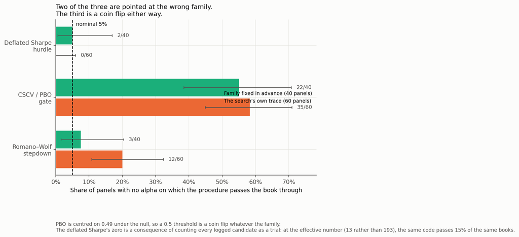
Realised size on a family fixed in advance against the search’s own trace
| Procedure | Family fixed in advance (40 panels) | The search’s own trace (60 panels) |
|---|---|---|
| Deflated Sharpe hurdle | 2 of 40 (5%) | 0 of 60 at N = 193 logged; 9 of 60 (15%) at N effective = 13 |
| CSCV / PBO gate | 22 of 40 (55%) | 35 of 60 (58%) |
| Romano–Wolf stepdown | 3 of 40 (8%) | 12 of 60 (20%) |
On a family chosen before the data I can detect no inflation in either formal procedure. Forty panels is not enough to certify a 5% test — the Romano–Wolf interval runs from 1.6% to 20.4% — so read that column as the absence of the gross inflation the search family produces, not as a calibration certificate. What is unambiguous is the other side. Pointed at the family the search produced, Romano–Wolf rejects on 12 of 60 panels containing nothing: four times nominal, binomial p < 10⁻⁴. Forty panels against sixty is too little to make the 8%-versus-20% contrast itself significant — Fisher’s exact test on that comparison gives p = 0.15 — so the claim that carries is the one against nominal, not the one across columns. The size inflation on the search family is also not a bootstrap artefact: it holds at expected block lengths of 5, 21 and 63 days and at 500 and 2,000 replications, ranging from 18% to 20% across all four settings.
Why? Not because the bootstrap fails to see the generations that bred the survivors — restrict the family to the search’s round-zero population, random expressions no selection has touched, and rejections fall from 12 panels to 6 (paired exact p = 0.07). That points at adaptive breeding as one contributor rather than the whole story; on sixty panels it is a direction, not a decomposition. The rest is the plainer fact that the family was chosen by looking at the window the test then uses.
The deflated Sharpe ratio is a more uncomfortable case, because its answer is determined by a number you supply. It needs the number of trials; I gave it the count of distinct expressions the search logged, a mean of 193 across panels (range 103 to 258). Those are not independent trials — the participation ratio of their correlation matrix averages 13 (range 5 to 26). Feeding 193 independent trials into a formula that assumes independence pushes the expected-maximum benchmark above the book’s Sharpe on 40 of 60 panels, and leaves the z-statistic short of the 95th percentile on the other twenty — so the hurdle rejects everything. Feed it 13 and the same code, on the same books, passes 9 of 60 — three times nominal (p = 0.003), in the opposite direction. The control’s verdict is a function of a modelling choice nobody documents. To be clear, no published implementation asks for an effective trial count; this is an extension of the method, not a correction to it.
And then there is PBO, which I had been treating as a control and which is not one. CSCV’s logit statistic is symmetric about zero when the candidate strategies are exchangeable and null, so the probability of backtest overfitting is centred on 0.49 — by construction, not by accident. A threshold at 0.5 is therefore a coin flip on data containing nothing: it passes 55% of pre-specified null books and 58% of searched null books. It is not powerless — against the strong plant it passes 95% — but a gate whose false-pass rate is 58% is not a 5% test, whatever it does on real signal.
4. What the controls cost you
Removing fiction is half of a control’s job. The other half is not destroying the thing you are looking for, and you cannot measure that on a null panel.
Against the strong plant — realised out-of-sample oracle Sharpe 2.43, above what the search can manufacture — here is what each control finds of it, alongside what it removes:
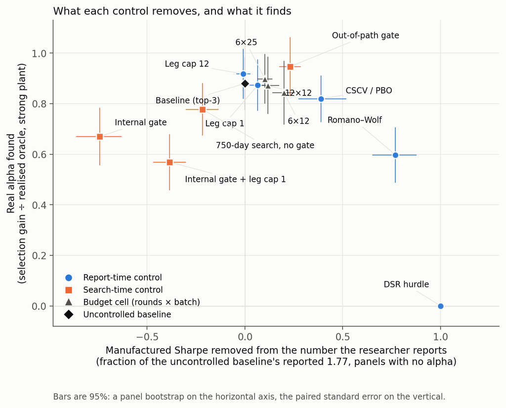
What each control removes and what it keeps
The right-hand column is the selection gain defined in the Setup — what selecting on the planted panel adds over what a null-selected book earns on it by construction. The raw ratio of book Sharpe to oracle is lower, because a book’s exposure to the plant is slightly negative on average: 0.81 for the baseline and 0.85 for the out-of-path gate.
| Control | Manufactured Sharpe removed | Real alpha found (selection gain ÷ oracle) |
|---|---|---|
| Out-of-path gate | 0.23 | 0.95 |
| Leg cap 12 | −0.01 | 0.92 |
| Budget 6 × 25 | 0.10 | 0.90 |
| Uncontrolled baseline | — | 0.88 |
| Leg cap 1 | 0.07 | 0.87 |
| Budget 12 × 12 | 0.12 | 0.87 |
| Budget 6 × 12 | 0.20 | 0.84 |
| CSCV / PBO gate | 0.39 | 0.82 |
| 750-day search, no gate | −0.22 | 0.78 |
| Internal gate | −0.74 | 0.67 |
| Romano–Wolf stepdown | 0.77 | 0.60 |
| Internal gate + leg cap 1 | −0.38 | 0.57 |
| Deflated Sharpe hurdle | 1.00 | 0.00 |
The minimum difference detectable at 80% power between the baseline and any of the seven pre-registered controls in that column, after Holm across the whole 84-test scan, runs from 0.05 to 0.21 of the oracle. Differences smaller than that should not be read — including the gap between the out-of-path gate’s 0.95 and the uncontrolled baseline’s 0.88, which is nominally the largest in the table and is not separable at this sample size.
The deflated Sharpe hurdle rejects a genuine 2.4-Sharpe strategy on all sixty panels, and passes exactly one of the sixty carrying the weak plant. Its perfect score in the removal column and its zero in the retention column are the same fact stated twice. A control that abstains on everything is unfalsifiable on null data and useless on real data, and you cannot tell those two properties apart without running a planted arm.
Romano–Wolf is the most defensible trade in the table: it removes 77% of the fiction — by abstaining four times in five — and keeps 60% of a strong real signal. That is a real control with a real price, which is more than most of this column can claim.
The out-of-path gate keeps the most alpha while removing a real 23% of the fiction. It is the only control whose null-panel out-of-sample Sharpe is even marginally negative (−0.086, SE 0.045, 95% CI [−0.17, +0.00]) — a t of 1.9 in a scan across fourteen arms, and inside the residual-tilt bound I flagged in the Setup, so I would not lean on the sign.
Four controls dominate the internal gate on both axes after Holm adjustment: leg cap 1, leg cap 12, the out-of-path gate, and — awkwardly — the PBO gate I have just described as a coin flip. No other pair dominates. That a gate with no size control still dominates the internal gate says more about the internal gate than it does about PBO.
A fourteenth arm, the shorter search with a leg cap of 1, is in the repository and not in these tables: it reports 2.01 on null panels — a little less inflation than the window-matched arm’s 2.15 — and finds 0.78 of the plant, which is the window-matched arm’s figure to within noise.
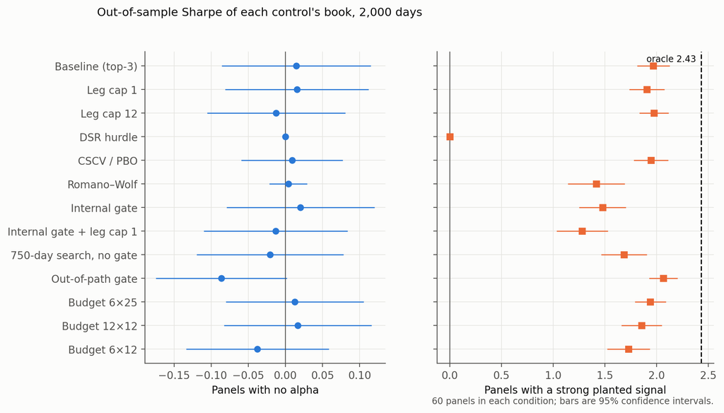
Out-of-sample Sharpe of each control’s book, with no alpha and with a strong plant
One more thing this table only shows because there is a strong plant in the study. Against the weak plant — oracle 0.59 — the uncontrolled pipeline’s selection gain is 11% of the oracle with a minimum detectable effect of 27%. That is not a finding, it is a non-detection, and the first pass of this study reported it as “the search captures 6% of the real signal”. The honest version is conditional and worth stating precisely: a search that ranks on in-sample Sharpe finds real alpha when the real alpha is larger than the alpha it can manufacture, and there is no evidence either way when it is smaller.
5. The agent behaves much like the machine
Eighteen fresh runs of the September research agent through a gated harness, six per condition, with the prompt frozen:
| Condition | Reported in-sample | Realised out-of-sample | Oracle | Found the plant |
|---|---|---|---|---|
| No alpha | 1.41 | −0.16 (SE 0.12) | — | — |
| Weak plant | 1.52 | +0.24 (SE 0.17) | 0.50 | 3 of 6 exactly, 4 of 6 by family |
| Strong plant | 2.91 | +2.04 (SE 0.16) | 2.31 | 3 of 6 exactly, 6 of 6 by family |
Manufactures on nothing, indistinguishable from noise against a weak signal, and its book earns 88% of the strong plant’s oracle out of sample against the mechanical pipeline’s 81% on the same raw basis. The arms ran on different panels and are not formally compared; qualitatively, whatever an LLM researcher is doing, it is not different enough from an evolutionary search to warrant a different control regime.
The arm is not blinded: the run id the agent types on every harness call carries the condition, K0, K1 or K2. Nothing in the logs refers to it, but it was in front of the agent, and six runs per condition is a small arm.
Two details worth having. The agents worked harder when there was more to find — 4.2 evaluation batches of a permitted 12 against the weak plant, 8.5 against the strong one — but they did not stop early on the null panel, where they used 5.7 batches and one run burned all twelve. That is responsiveness to signal strength, not an ability to notice there is nothing there.
And the twelve September agent traces, re-scored under the report-time controls on drift-free panels, behave as the mechanical arms do: the deflated Sharpe hurdle passes 0 of 12, PBO 5 of 12, Romano–Wolf 7 of 12. The exception is leg caps, which move an agent’s reported Sharpe by +0.02 on average at a cap of one and −0.02 at a cap of twelve — never by more than 0.29 on any single run, and in no consistent direction — because an agent’s legs live inside a single expression rather than in the count of expressions. Any control that counts expressions is close to blind to an agent.
6. One real path, for illustration
The same pipeline on a real panel — 1,280 NASDAQ names, search 2018–2020, holdout 2021 [5]. One path, a stale and survivorship-conditioned dataset, and a universe filter that looks at the whole sample. It evidences nothing; it is here because it makes the synthetic result legible.
| Book | In-sample 2018–2020 | Holdout 2021 | Through May 2023 |
|---|---|---|---|
| Baseline (top-3) | +2.57 | −0.41 | −0.24 |
| Leg cap 1 | +2.11 | −0.56 | −0.45 |
| Leg cap 12 | +2.00 | −0.45 | −0.26 |
| CSCV / PBO (passed) | +2.57 | −0.41 | −0.24 |
| Internal gate | +1.94 | −0.47 | −0.26 |
| Internal gate + leg cap 1 | +2.11 | −0.56 | −0.45 |
| Budget 6 × 25 | +1.85 | −0.61 | −0.52 |
| Budget 12 × 12 | +2.40 | −0.21 | −0.30 |
| Budget 6 × 12 | +1.54 | −0.73 | −0.64 |
| Deflated Sharpe hurdle | abstained | — | — |
| Romano–Wolf | abstained | — | — |
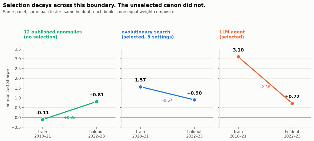
| Twelve published anomalies, no selection | −0.40 | +0.69 | +0.69 |
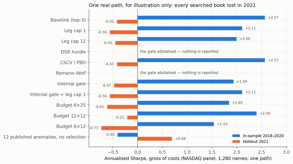
Every searched book on the real panel, in sample and out
Every searched book turned negative. The unselected canon, which looked worst in sample, was the only thing that worked out of sample. Consistent with the synthetic result, and worth precisely as much as one path is worth.
One inconsistency to flag rather than let a reader find: the in-sample column here is the full 2018–2020 window for every book, including the internal gate, so it is not the reported-window number section 2 corrects to. On this arm the gate therefore appears to lower the in-sample figure when the synthetic result says it raises the number the gate’s user would report. The real panel’s dataset is fetched over the network and I could not re-score that row from the sandbox this study ran in; it is stated here rather than quietly left in the table.
The pre-registration scorecard
| Prediction | Verdict |
|---|---|
| P1 the out-of-path gate dominates the DSR hurdle on both axes | Refuted, with each control winning one axis: the out-of-path gate removes 1.36 less of the reported Sharpe (CI [−1.45, −1.27]) and finds 2.07 more of the plant (CI [+1.92, +2.21]) |
| P2 a leg cap of 1 removes ≥ 0.20 more than the smallest budget cell | Refuted: −0.13, CI [−0.19, −0.07] |
| P3 the DSR hurdle’s size exceeds 25% | Refuted: 0 of 60, conditional on N = logged candidates |
| P4a the internal gate costs ≥ 0.10 Sharpe on planted panels | Confirmed: −0.49, CI [−0.69, −0.29] |
| P4b the internal gate removes ≥ 0.50 of the manufactured Sharpe | Refuted, and in the opposite direction: −0.74 |
Things that did not work
The leg axis. Capping a book at one leg removes 0.13 less manufactured Sharpe than the smallest search budget does — the budget axis beat the leg axis, and leg caps are close to a no-op on this pipeline. Against an agent they are a complete no-op, for the reason in section 5. This is the one place where I expected a result from the literature to transfer and it didn’t: in-sample statistics do inflate with the number of combined signals [9], but not in a way a cap on the count can reach when the signals are themselves sums.
The pre-registered “oracle frontier” — thresholding candidates on their true out-of-sample Sharpe to trace the best attainable trade-off — is not reported at all. Estimating “true” out-of-sample Sharpe on the same window that scores the books is circular, and on null panels it obligingly produced a frontier that “retained” +0.60 of Sharpe that does not exist. The file is in the repository; the chart does not draw it.
And the first version of this study, which four reviewers took apart before publication. The largest correction was measuring each control on the number a researcher reports rather than the number they discard, which reversed the sign of the headline. The second was noticing that my planted signal had been calibrated to a level the search could beat by fabrication, which made one of my conclusions a property of the experiment rather than of the world. The third was catching three numbers quoted from the weak-plant arm where the text said otherwise. The fourth was showing that this post’s own draft compared the random family and the search on different windows, which inflated the gap in section 1 into a result it is not. All eighteen deviations are logged, and the first-pass tables sit in the repository beside the corrected ones.
What this does and does not show
It does show that on a verified-null panel an in-sample Sharpe of about 1.9 comes out of selecting three candidates from a couple of hundred, on the window the selection is made, and that twelve rounds of adaptive search add nothing measurable to that number.
It does show that a held-out validation window, used the way it is normally used, raises the reported Sharpe rather than lowering it, by roughly the factor the standard error of a Sharpe estimate predicts; and that a fresh-path re-test mostly relocates the manufactured Sharpe rather than removing it.
It does show that two of the three formal procedures show no detectable inflation on a family fixed in advance and are grossly mis-sized on a family the search selected; and that the third is centred on its own threshold under the null and therefore does not decide anything about size.
It does show that a pipeline, mechanical or agentic, recovers most of a planted signal strong enough to beat what it can manufacture — and that the deflated Sharpe hurdle, as conventionally parameterised, destroys all of it.
It does not show that any of these procedures is wrong. Each is implemented here against its published definition and is doing what it was designed to do on the input it is handed.
It does not show anything about faint alpha. Against a signal with a 0.59 oracle Sharpe this design cannot separate “finds nothing” from “finds a quarter of it”. That needs more panels or a longer scoring window.
It does not show a ranking of controls that transfers. The removal axis depends on the reporting convention, the retention axis on a plant that happens to be a single expression the grammar can write exactly — evaluated verbatim by the mechanical search on only 6 of the 60 strong-plant panels, so its findability is not an artefact of expressibility, but a plant the grammar cannot write at all would give a different answer. The leg-cap results depend on a grammar in which a leg is a separate expression, and every net-of-cost number on a book volatility of about 2.5%.
It does not show anything about real markets. One path on a stale dataset is an illustration.
So what do you do?
Report the number you selected on, and say which window it is. Most of the apparent power of every re-selection control in this study came from measuring it on a window the researcher had already discarded: the out-of-path gate’s removal falls from 0.99 to 0.23 when you do this properly, and the internal gate’s flips sign, from +0.47 to −0.74. If your validation split produces a Sharpe of 3.1 where your in-sample fit produced 1.8, the honest headline is 3.1, and the fact that it is larger should alarm you rather than reassure you.
Write down the family before you look. Not the trial count — the family. Every procedure in section 3 shows no inflation on a family fixed in advance and gross inflation on a family your search selected, and the difference between those is a decision you make before the data, not a correction you apply after it.
If you use the deflated Sharpe ratio, state how you counted trials, and report the effective number alongside the raw count. The gap between 193 and 13 on the same candidate set moved the pass rate from 0% to 15%. No published implementation asks for an effective count, so this is an extension rather than a fix — but a DSR quoted without saying how trials were counted is a number with a free parameter in it.
Stop using a PBO threshold of 0.5 as a gate. It is centred on 0.49 under the null. Use the distribution, or use something else.
Run a planted arm. This is the one that costs real effort and is worth it. A control that abstains on everything looks perfect on a null panel; you only find out what it costs when you give it something real to find. And calibrate the plant above what your own pipeline can fabricate, or you will measure your calibration rather than your control — which is exactly what the first version of this study did.
Code and data
The repository holds the pre-registered analysis plan committed before the first run, eighteen logged deviations from it, the corrected generator with its bitwise verification against the September panels, the calibration of both plants, the full study across 180 panels, the pre-specified-family placebo, the erratum arithmetic against all 294 previously published books, the agent harness with every run log and journal, the canary tests, and the analysis and figure code. Seeds: study panels 9000–9059, calibration 8000–8029, placebo panels 9500–9539, pre-specified family drawn from seed 20260921. Everything except the LLM calls reproduces from those seeds; the LLM calls are not re-runnable, which is why the logs are included in full. The repository is at github.com/jkinlay/research-controls; this article refers to commit c11241e.
Two requests of anyone re-running it. Fix your family before you look at the data, and keep the list. And run a planted arm alongside the null arm — half the results here are invisible without one.
References
[1] Bailey & López de Prado, The Deflated Sharpe Ratio: Correcting for Selection Bias, Backtest Overfitting and Non-Normality, Journal of Portfolio Management 40(5), 2014.
[2] Bailey, Borwein, López de Prado & Zhu, The Probability of Backtest Overfitting, Journal of Computational Finance 20(4), 2017; and Pseudo-Mathematics and Financial Charlatanism, Notices of the AMS 61(5), 2014, for the expected-maximum-Sharpe result.
[3] Romano & Wolf, Stepwise Multiple Testing as Formalized Data Snooping, Econometrica 73(4), 2005, 1237–1282. The stepdown implemented here is the one-sided studentised version at 5% familywise error.
[4] Politis & Romano, The Stationary Bootstrap, Journal of the American Statistical Association 89(428), 1994. Expected block length 21 days throughout. The section 3 size result is stable across that choice: 18% at a block length of 5, 20% at 21, 18% at 63, and 18% at 21 with 2,000 replications rather than 500.
[5] skfolio, load_nasdaq_dataset — daily adjusted closes, 1,455 NASDAQ constituents, 2018-01-02 to 2023-05-31, documented by its authors as a stale dataset not intended for investment or commercial use. Filtered here to 1,280 names with median price ≥ $5.
[6] Harvey & Liu, Backtesting, Journal of Portfolio Management 42(1), 2015 — the multiple-testing haircut the report-time controls in section 3 descend from.
[7] Harvey & Liu, False (and Missed) Discoveries in Financial Economics, Journal of Finance 75(5), 2020, on the two-sided cost of correction; section 4 is a direct measurement of the missed-discovery side. See also Chen, The Limits of p-Hacking: Some Thought Experiments, Journal of Finance 76(5), 2021, 2447–2480, for the argument that selection alone cannot account for the observed cross-section — the complement of the measurement in section 1.
[8] Dwork, Feldman, Hardt, Pitassi, Reingold & Roth, The reusable holdout: Preserving validity in adaptive data analysis, Science 349(6248), 2015. Section 2 is the practical, one-reuse form of the result that a holdout used for selection stops being a holdout.
[9] Novy-Marx, Backtesting Strategies Based on Multiple Signals, NBER Working Paper 21329, 2015, on the inflation of in-sample statistics with the number of combined signals — the leg axis that section 4 finds to be a no-op here.
Disclosure: I run systematic strategies. Nothing here is a recommendation, and no strategy discussed is one I trade. These are diagnostic quantities from a methodological experiment on synthetic data and one stale public dataset, not a track record.