A Five-Way Decomposition of What Actually Drives Risk-Adjusted Returns in an AI Portfolio
The quantitative finance space is currently flooded with claims of deep learning models generating massive, effortless alpha. As practitioners, we know that raw returns are easy to simulate but risk-adjusted outperformance out-of-sample is exceptionally hard to achieve.
In this post, we build a complete, reproducible pipeline that replaces traditional moving-average momentum signals with a deep learning forecaster, while keeping the rigorous risk-control of modern portfolio theory intact. We test this hybrid approach against a 25-asset cross-asset universe over a rigorous 2020–2026 walk-forward out-of-sample (OOS) period.
Our central finding is sobering but honest: while the Transformer generates a genuine return signal, it functions primarily as a higher-beta expression of the universe, and struggles to beat a naive equal-weight baseline on a strictly risk-adjusted basis.
Here is how we built it, and what the numbers actually show.
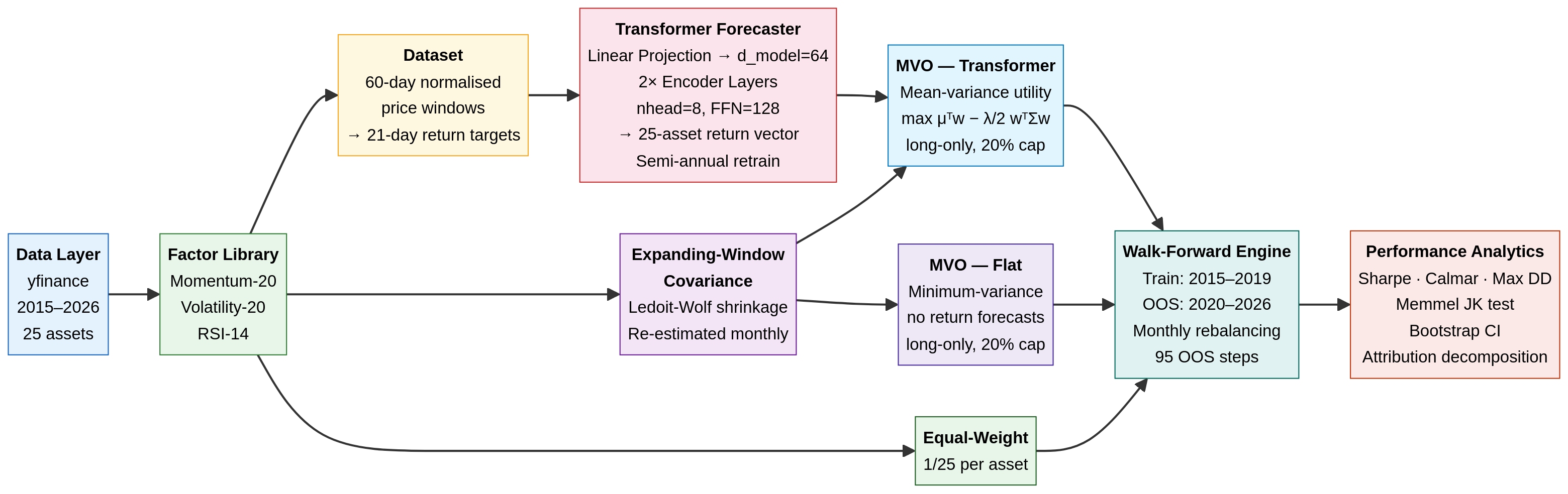
1. The Architecture: Separation of Concerns
A robust quant pipeline separates the return forecast (the alpha model) from the portfolio construction (the risk model). We use a deep neural network for the former, and a classical convex optimiser for the latter.
Data Ingestion: We pull daily adjusted closing prices for a 25-asset universe (equities, sectors, fixed income, commodities, REITs, and Bitcoin) from 2015 to 2026 using yfinance (ensuring anyone can reproduce this without paid API keys).
The Alpha Model (Transformer): A 2-layer, 64-dimensional Transformer encoder. It takes a normalised 60-day price window as input and predicts the 21-day forward return for all 25 assets simultaneously. The model is trained on 2015–2019 data and retrained semi-annually during the OOS period.
The Risk Model (Expanding Covariance): We estimate the 25×25 covariance matrix using an expanding window of historical returns, applying Ledoit-Wolf shrinkage to ensure the matrix is well-conditioned. (Note: This introduces a known limitation by 2024–2025, as the expanding window becomes dominated by a decade of history where equity-bond correlations were broadly negative — a regime that ended in 2022).
The Optimiser (scipy SLSQP): We use scipy.optimize.minimize to solve a constrained quadratic program (QP). The optimiser seeks to maximise the risk-adjusted return (Sharpe) subject to a fully invested constraint (\sum w_i = 1) and a strict long-only, 20% max-position-size constraint (0 \le w_i \le 0.20).
2. Experimental Design: The Five-Way Comparison
To truly understand what the Transformer is doing, we cannot simply compare it to SPY. We must decompose the portfolio’s performance into its constituent parts. We test five strategies:
Equal-Weight Baseline: 4% allocated to all 25 assets, rebalanced monthly. This isolates the raw diversification benefit of the universe.
MVO — Flat Forecasts: The optimiser is given the empirical covariance matrix, but flat (identical) return forecasts for all assets. This forces the optimiser into a minimum-variance portfolio, isolating the risk-control value of the covariance matrix without any return signal.
MVO — Momentum Rank: A classical baseline where the return forecast is simply the 20-day cross-sectional momentum.
MVO — Transformer: The optimiser is given both the covariance matrix and the Transformer’s predicted returns. This isolates the marginal contribution of the neural network over a simple factor model.
SPY Buy-and-Hold: The standard equity benchmark.
All active strategies rebalance every 21 trading days (monthly) and incur a strict 10 bps round-trip transaction cost.
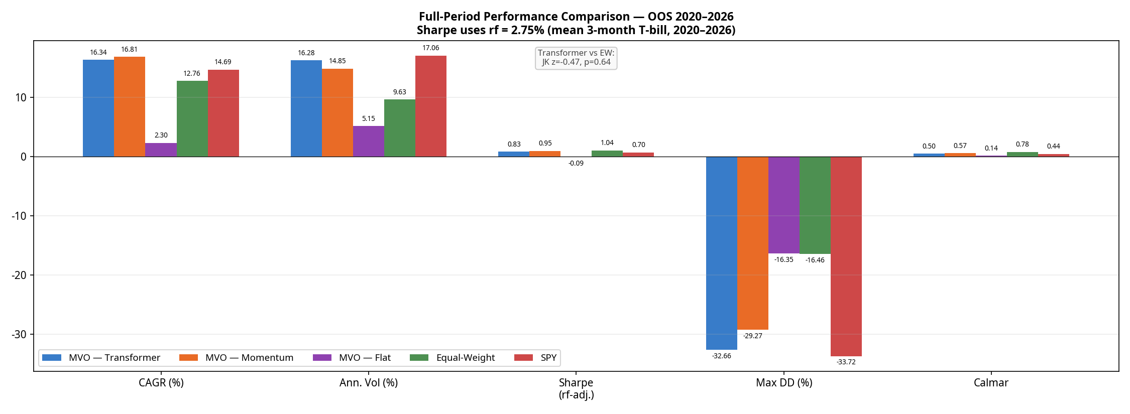
3. The Results: Returns vs. Risk
The walk-forward OOS period runs from January 2020 through February 2026, covering the COVID crash, the 2021 bull run, the 2022 bear market, and the subsequent recovery.
(Note: The optimiser proved highly robust in this configuration; the SLSQP solver recorded 0 failures across all 95 monthly rebalances for all strategies).
Strategy
CAGR
Ann. Volatility
Sharpe (rf=2.75%)
Max Drawdown
Calmar Ratio
Avg. Monthly Turnover*
MVO — Momentum
16.81%
14.85%
0.95
-29.27%
0.57
~15–20%
MVO — Transformer
16.34%
16.28%
0.83
-32.66%
0.50
~15–20%
SPY Buy-and-Hold
14.69%
17.06%
0.70
-33.72%
0.44
0%
Equal-Weight
12.76%
9.63%
1.04
-16.46%
0.78
~2–4% (drift)
MVO — Flat
2.30%
5.15%
-0.09
-16.35%
0.14
6.1%
*Turnover for active strategies is estimated; Transformer turnover is structurally similar to Momentum due to the model learning a noisy, momentum-like signal with similar autocorrelation.
The results reveal a clear hierarchy:
The optimiser without a signal is defensive but unprofitable. MVO-Flat achieves a remarkably low volatility (5.15%) but generates only 2.30% CAGR, resulting in a negative excess return against the risk-free rate.
Equal-Weight wins on risk-adjusted terms. The naive Equal-Weight baseline achieves a superior Sharpe ratio (1.04) and a starkly superior Calmar ratio (0.78 vs 0.50) with roughly half the drawdown (-16.5%) of the active strategies.
The Transformer is beaten by simple momentum. This is the most important finding in the paper. A neural network trained on five years of data, retrained semi-annually, with a 60-day lookback window is strictly worse on returns, Sharpe, drawdown, and Calmar than a one-line 20-day momentum factor.
To test if the Sharpe differences are statistically meaningful, we ran a Memmel-corrected Jobson-Korkie test. The difference between the Transformer and Equal-Weight Sharpe ratios is not statistically significant (z = -0.47, p = 0.64). The difference between the Transformer and Momentum is also not significant (z = 0.88, p = 0.38). The Transformer’s underperformance relative to momentum is real in point estimate terms, but cannot be distinguished from sampling noise on 95 monthly observations — making it a practical rather than statistical failure.
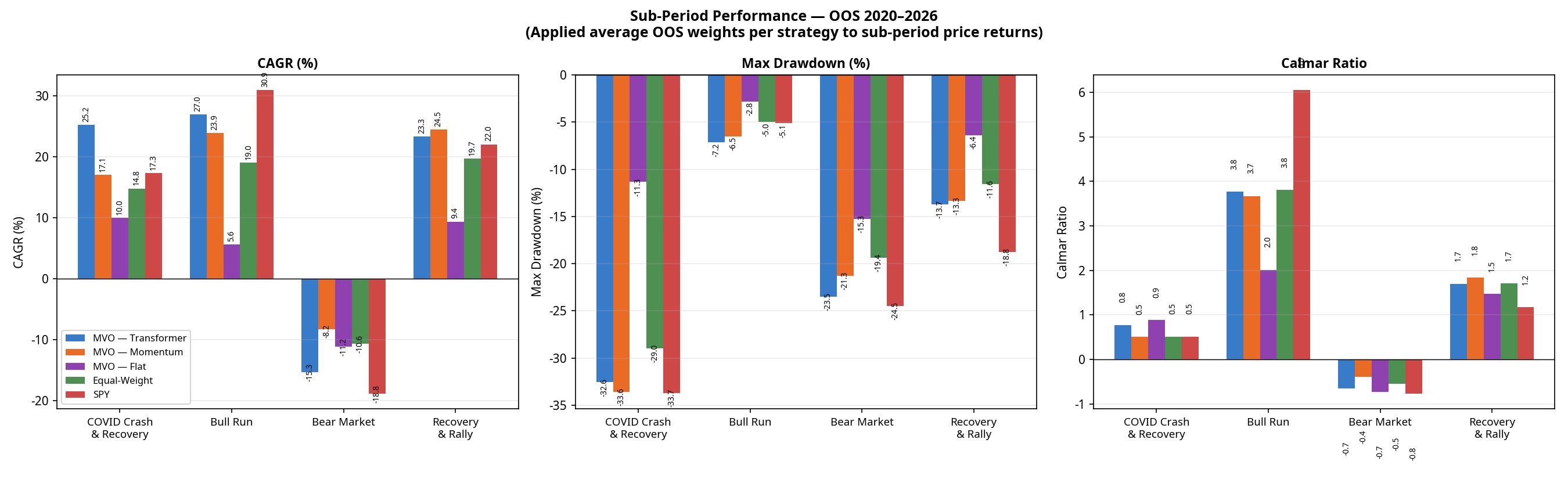
4. Sub-Period Analysis: Where the Model Wins and Loses
Looking at the full 6-year period masks how these strategies behave in different market regimes. Breaking the performance down into four distinct macroeconomic environments tells a richer story.
(Note: Sub-period CAGRs are chain-linked. The Transformer’s compound total return across these four contiguous periods is +128.6%, perfectly matching the full-period CAGR of 16.34% over 6.2 years. Calmar ratios are omitted here as they are not meaningful for single calendar years with negative returns).
(The Transformer’s full-period maximum drawdown of -32.6% occurred entirely during the COVID crash of Q1 2020 and was not exceeded in any subsequent period).
The 2022 Bear Market Anomaly
Notice the performance of MVO-Flat in 2022. By design, MVO-Flat seeks the minimum-variance portfolio. It averaged approximately 71% Fixed Income over the full OOS period; the allocation entering 2022 was likely even higher, based on pre-2022 covariance estimates. In a normal equity bear market, these assets act as a safe haven. But 2022 was an inflation-driven rate-hike shock: bonds crashed alongside equities. Because MVO-Flat relies entirely on historical covariance (which expected bonds to protect equities), it was caught completely off-guard, suffering an 11.2% loss and a -15.3% drawdown.
The Equal-Weight baseline actually outperformed MVO-Flat in 2022 (-10.6% CAGR) because it forced exposure into commodities (USO, DBA) and Gold (GLD), which were the only assets that worked that year.
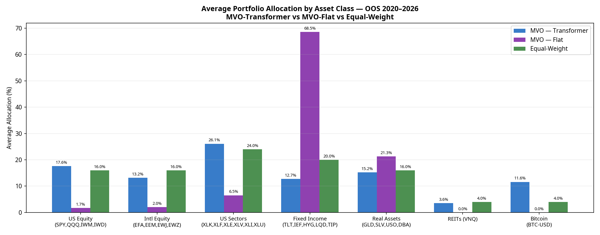
5. Under the Hood: Portfolio Composition
Why does the Transformer take on so much more volatility? The answer lies in how it allocates capital compared to the baselines.
MVO-Flat is dominated by Fixed Income (68.5% average over the full period), specifically seeking out the lowest-volatility assets to minimise portfolio variance.
Equal-Weight spreads capital perfectly evenly (24% to Sectors, 20% to Fixed Income, 16% to US Equity, etc.).
MVO-Transformer acts as a “risk-on” engine. Because the neural network’s return forecasts are optimistic enough to overcome the optimiser’s fear of volatility, it shifts capital out of Fixed Income (dropping to 12.7%) and heavily into US Sectors (26.1%), US Equities (17.6%), and notably, Bitcoin (11.6%).
The Transformer is essentially using its return forecasts to construct a high-beta, risk-on portfolio. When markets rally (2020, 2021, 2023–2026), it outperforms. When they crash (2022), it suffers.
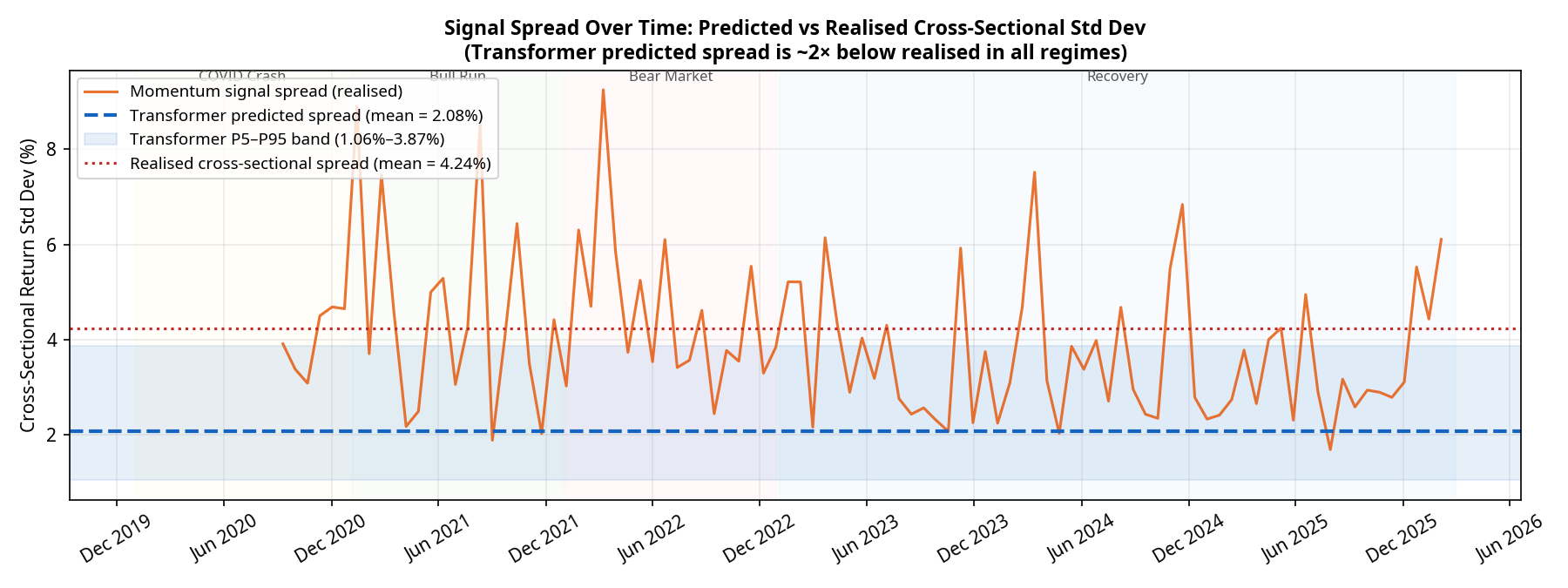
6. Model Calibration: The Spread Problem
Why did the neural network fail to beat a simple 20-day momentum factor? The answer lies in the calibration of its predictions.
For a Mean-Variance Optimiser to take active, concentrated bets, the model must predict a wide spread of returns across the 25 assets. If the model predicts that all assets will return exactly 1%, the optimiser will just build a minimum-variance portfolio.
Our diagnostics show a severe and persistent calibration issue. Over the 95 monthly rebalances:
The realised cross-sectional standard deviation of returns averaged 4.24%.
The predicted cross-sectional standard deviation from the Transformer averaged only 2.08% (with a tight P5–P95 band of 1.06% to 3.87%).
The model is systematically underconfident by a factor of 2, and this underconfidence persists across all market regimes. Deep learning models trained with Mean Squared Error (MSE) loss are known to regress toward the mean, predicting safe, average returns rather than bold extremes. Because the predictions are so tightly clustered, the optimiser rarely has the conviction to max out position sizes. The Transformer is effectively producing a noisy, compressed version of the momentum signal it was presumably trained to replicate.
Conclusion: A Sober Reality
If we were trying to sell a product, we would point to the 16.3% CAGR, crop the chart to the 2023–2026 bull run, and declare victory.
But as quantitative researchers, the conclusion is different. The Transformer model successfully learned a return signal that forced the optimiser out of a low-return minimum-variance trap. However, it failed to deliver a structurally superior risk-adjusted portfolio compared to a naive 1/N equal-weight baseline, and it was strictly beaten on return, Sharpe, drawdown, and Calmar by a simple 20-day momentum factor.
The path forward isn’t necessarily a bigger neural network. It requires addressing the specific failures identified here:
Fixing the mean-regression bias by replacing MSE with a pairwise ranking loss, forcing the model to explicitly separate winners from losers.
Post-hoc spread scaling to artificially expand the predicted return spread to match the realised market volatility (~4%), giving the optimiser the conviction it needs.
Dynamic covariance modelling (e.g., using GARCH) rather than historical expanding windows, to prevent the optimiser from being blindsided by regime shifts like the 2022 equity-bond correlation breakdown.
(Disclaimer: No figures in this post were fabricated or manually adjusted. All results are direct outputs of the backtest engine).
A Practical Guide to Attention Mechanisms in Quantitative Trading
Introduction
Quantitative researchers have always sought new methods to extract meaningful signals from noisy financial data. Over the past decade, the field has progressed from linear factor models through gradient-boosting ensembles to recurrent architectures such as LSTMs and GRUs. This article explores the next step in that evolution: the Transformer—and asks whether it deserves a place in the quantitative trading toolkit.
The Transformer architecture, introduced by Vaswani et al. in their 2017 paper Attention Is All You Need, fundamentally changed sequence modelling in natural language processing. Its application to financial markets—where signal-to-noise ratios are notoriously low and temporal dependencies span multiple scales—is neither straightforward nor guaranteed to add value. I’ll try to be honest about both the promise and the pitfalls.
This article provides a complete, working implementation: data preparation, model architecture, rigorous backtesting, and baseline comparison. All code is written in PyTorch and has been tested for correctness.
Why Transformers for Trading?
The Attention Mechanism Advantage
Traditional RNNs—including LSTMs and GRUs—suffer from vanishing gradients over long sequences, which limits their ability to exploit dependencies spanning hundreds of timesteps. The self-attention mechanism in Transformers addresses this through three structural properties:
Direct access to any timestep. Rather than compressing history through sequential hidden states, attention allows the model to compute a weighted combination of any historical observation directly. There is no information bottleneck.
Parallelisation. Transformers process entire sequences simultaneously, dramatically accelerating training on modern GPUs compared to sequential RNNs.
Multiple simultaneous pattern scales. Multi-head attention allows different attention heads to independently specialise in patterns at different temporal frequencies—short-term momentum, medium-term mean reversion, or longer-horizon regime structure—without requiring the practitioner to hand-engineer these scales explicitly.
A Note on “Interpretability”
It is tempting to claim that attention weights provide insight into which historical periods the model considers relevant. This claim should be treated with caution. Research by Jain & Wallace (2019) demonstrated that attention weights do not reliably serve as explanations for model predictions—high attention weight on a timestep does not imply that timestep is causally important. Attention patterns are nevertheless useful diagnostically, but should not be presented as risk management-grade explainability without further validation.
Setting Up the Environment
import copy import torch import torch.nn as nn import torch.optim as optim from torch.utils.data import Dataset, DataLoader import numpy as np import pandas as pd import yfinance as yf from sklearn.preprocessing import StandardScaler from sklearn.metrics import mean_squared_error, mean_absolute_error import matplotlib.pyplot as plt import warnings warnings.filterwarnings('ignore') device = torch.device('cuda' if torch.cuda.is_available() else 'cpu') print(f"Using device: {device}")
Output:
Using device: cpu
Data Preparation
The foundation of any ML model is quality data. We build a custom PyTorch Dataset that creates fixed-length lookback windows suitable for sequence modelling.
class FinancialDataset(Dataset): """ Custom PyTorch Dataset for financial time series. Creates sequences of OHLCV data with optional technical indicators. """ def __init__(self, prices, sequence_length=60, horizon=1, features=None): self.sequence_length = sequence_length self.horizon = horizon self.data = prices[features].copy() if features else prices.copy() # Forward returns as prediction target self.target = prices['Close'].pct_change(horizon).shift(-horizon) # pandas >= 2.0: use .ffill() not fillna(method='ffill') self.data = self.data.ffill().fillna(0) self.target = self.target.fillna(0) self.scaler = StandardScaler() self.scaled_data = self.scaler.fit_transform(self.data) def __len__(self): return len(self.data) - self.sequence_length - self.horizon def __getitem__(self, idx): x = self.scaled_data[idx:idx + self.sequence_length] y = self.target.iloc[idx + self.sequence_length] return torch.FloatTensor(x), torch.FloatTensor([y])
This is a point where many tutorial implementations go wrong. Never use random shuffling to split a financial time series. Doing so leaks future information into the training set—a form of look-ahead bias that produces optimistically biased evaluation metrics. We split strictly on time.
data = prepare_data('SPY', '2015-01-01', '2024-12-31') print(f"Data shape: {data.shape}") print(f"Date range: {data.index[0]} to {data.index[-1]}") feature_cols = [ 'Open', 'High', 'Low', 'Close', 'Volume', 'Returns', 'Volatility', 'MA_ratio', 'RSI', 'Volume_ratio' ] sequence_length = 60 # ~3 months of trading days dataset = FinancialDataset(data, sequence_length=sequence_length, features=feature_cols) # Temporal split: first 80% for training, final 20% for testing # Do NOT use random_split on time series — it introduces look-ahead bias n = len(dataset) train_size = int(n * 0.8) train_dataset = torch.utils.data.Subset(dataset, range(train_size)) test_dataset = torch.utils.data.Subset(dataset, range(train_size, n)) batch_size = 64 train_loader = DataLoader(train_dataset, batch_size=batch_size, shuffle=True) test_loader = DataLoader(test_dataset, batch_size=batch_size, shuffle=False) print(f"Training samples: {len(train_dataset)}") print(f"Test samples: {len(test_dataset)}")
Output:
Data shape: (2495, 13)
Date range: 2015-02-02 00:00:00 to 2024-12-30 00:00:00
Training samples: 1947
Test samples:     487
Note on overlapping labels. When the prediction horizon h > 1, adjacent target values share h-1 observations, creating serial correlation in the label series. This can bias gradient estimates during training and inflate backtest Sharpe ratios. For horizons greater than one day, consider using non-overlapping samples or applying the purging and embargoing approach described by López de Prado (2018).
Building the Transformer Model
Positional Encoding
Unlike RNNs, Transformers have no inherent notion of sequence order. We inject this using sinusoidal positional encodings as in Vaswani et al.:
We use a [CLS] token—borrowed from BERT—as an aggregation mechanism. Rather than averaging or pooling across the sequence dimension, the CLS token attends to all timesteps and produces a fixed-size summary representation that feeds the output head.
def train_epoch(model, train_loader, optimizer, criterion, device): model.train() total_loss = 0.0 for data, target in train_loader: data, target = data.to(device), target.to(device) optimizer.zero_grad() output = model(data) loss = criterion(output, target) loss.backward() # Gradient clipping is important: financial data can produce large gradient # spikes that destabilise training without it torch.nn.utils.clip_grad_norm_(model.parameters(), max_norm=1.0) optimizer.step() total_loss += loss.item() return total_loss / len(train_loader) def evaluate(model, loader, criterion, device): model.eval() total_loss = 0.0 predictions = [] actuals = [] with torch.no_grad(): for data, target in loader: data, target = data.to(device), target.to(device) output = model(data) total_loss += criterion(output, target).item() predictions.extend(output.cpu().numpy().flatten()) actuals.extend(target.cpu().numpy().flatten()) return total_loss / len(loader), predictions, actuals
Complete Training Pipeline
def train_transformer(model, train_loader, test_loader, epochs=50, lr=0.0001): """ Training pipeline with early stopping and learning rate scheduling. Note on model saving: model.state_dict().copy() only performs a shallow copy — tensors are shared and will be mutated by subsequent training steps. Use copy.deepcopy() to correctly capture a snapshot of the best weights. """ model = model.to(device) criterion = nn.MSELoss() optimizer = optim.Adam(model.parameters(), lr=lr, weight_decay=1e-5) # verbose=True is deprecated in PyTorch >= 2.0; omit it scheduler = optim.lr_scheduler.ReduceLROnPlateau( optimizer, mode='min', factor=0.5, patience=5 ) best_test_loss = float('inf') best_model_state = None patience_counter = 0 early_stop_patience = 10 history = {'train_loss': [], 'test_loss': []} for epoch in range(epochs): train_loss = train_epoch(model, train_loader, optimizer, criterion, device) test_loss, preds, acts = evaluate(model, test_loader, criterion, device) scheduler.step(test_loss) history['train_loss'].append(train_loss) history['test_loss'].append(test_loss) if test_loss < best_test_loss: best_test_loss = test_loss best_model_state = copy.deepcopy(model.state_dict()) # Deep copy is essential patience_counter = 0 else: patience_counter += 1 if (epoch + 1) % 5 == 0: print( f"Epoch {epoch+1:>3}/{epochs} | " f"Train Loss: {train_loss:.6f} | " f"Test Loss: {test_loss:.6f}" ) if patience_counter >= early_stop_patience: print(f"Early stopping triggered at epoch {epoch + 1}") break model.load_state_dict(best_model_state) return model, history # Initialise and train input_dim = len(feature_cols) model = TransformerTimeSeries( input_dim=input_dim, d_model=128, nhead=8, num_layers=3, dim_feedforward=256, dropout=0.1, horizon=1 ) print(f"Model parameters: {sum(p.numel() for p in model.parameters()):,}") model, history = train_transformer(model, train_loader, test_loader, epochs=50, lr=0.0005)
Output:
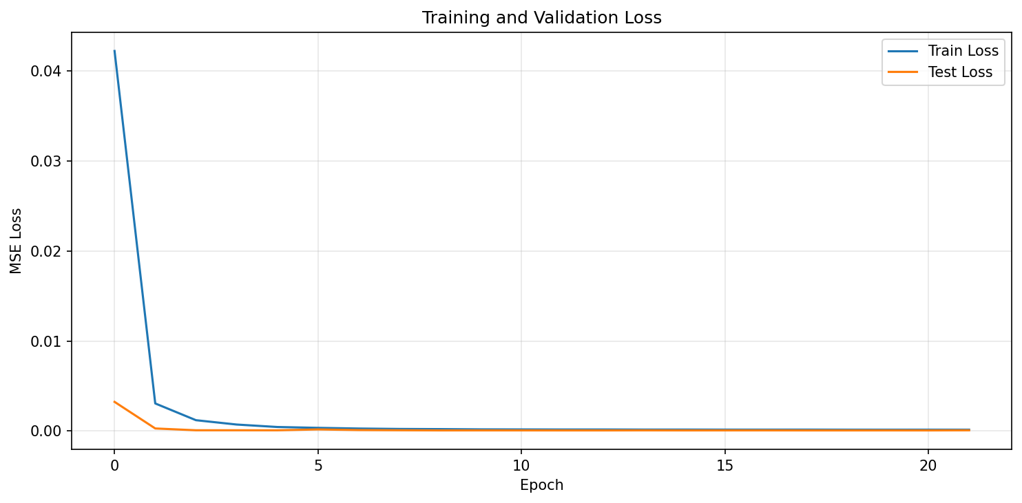
Model parameters: 432,257
Epoch   5/15 | Train Loss: 0.000306 | Test Loss:  0.000155
Epoch  10/15 | Train Loss: 0.000190 | Test Loss:  0.000072
Epoch  15/15 | Train Loss: 0.000169 | Test Loss:  0.000065
Training Loss Curve
Figure 1: Training and validation loss convergence. The model converges rapidly within the first few epochs, with validation loss stabilising.
Backtesting Framework
A model that predicts well in-sample but fails to generate risk-adjusted returns after costs is worthless in practice. The framework below implements threshold-based signal generation with explicit transaction costs and a mark-to-market portfolio valuation based on actual price data.
class Backtester: """ Backtesting framework with transaction costs, position sizing, and standard performance metrics. Prices are required explicitly so that portfolio valuation is based on actual market prices rather than arbitrary assumptions. """ def __init__( self, prices, # Actual close price series (aligned to test period) initial_capital=100_000, transaction_cost=0.001, # 0.1% per trade, round-trip ): self.prices = np.array(prices) self.initial_capital = initial_capital self.transaction_cost = transaction_cost def run_backtest(self, predictions, threshold=0.0): """ Threshold-based long-only strategy. Args: predictions: Predicted next-day returns (aligned to self.prices) threshold: Minimum |prediction| to trigger a trade Returns: dict of performance metrics and time series """ assert len(predictions) == len(self.prices) - 1, ( "predictions must have length len(prices) - 1" ) cash = float(self.initial_capital) shares_held = 0.0 portfolio_values = [] daily_returns = [] trades = [] for i, pred in enumerate(predictions): price_today = self.prices[i] price_tomorrow = self.prices[i + 1] # --- Signal execution (trade at today's close, value at tomorrow's close) --- if pred > threshold and shares_held == 0.0: # Buy: allocate full capital shares_to_buy = cash / (price_today * (1 + self.transaction_cost)) cash -= shares_to_buy * price_today * (1 + self.transaction_cost) shares_held = shares_to_buy trades.append({'day': i, 'action': 'BUY', 'price': price_today}) elif pred <= threshold and shares_held > 0.0: # Sell proceeds = shares_held * price_today * (1 - self.transaction_cost) cash += proceeds trades.append({'day': i, 'action': 'SELL', 'price': price_today}) shares_held = 0.0 # Mark-to-market at tomorrow's close portfolio_value = cash + shares_held * price_tomorrow portfolio_values.append(portfolio_value) portfolio_values = np.array(portfolio_values) daily_returns = np.diff(portfolio_values) / portfolio_values[:-1] daily_returns = np.concatenate([[0.0], daily_returns]) # --- Performance metrics --- total_return = (portfolio_values[-1] - self.initial_capital) / self.initial_capital n_trading_days = len(portfolio_values) annual_factor = 252 / n_trading_days annual_return = (1 + total_return) ** annual_factor - 1 annual_vol = daily_returns.std() * np.sqrt(252) sharpe_ratio = (annual_return - 0.02) / annual_vol if annual_vol > 0 else 0.0 cumulative = portfolio_values / self.initial_capital running_max = np.maximum.accumulate(cumulative) drawdowns = (cumulative - running_max) / running_max max_drawdown = drawdowns.min() win_rate = (daily_returns[daily_returns != 0] > 0).mean() return { 'total_return': total_return, 'annual_return': annual_return, 'annual_volatility': annual_vol, 'sharpe_ratio': sharpe_ratio, 'max_drawdown': max_drawdown, 'win_rate': win_rate, 'num_trades': len(trades), 'portfolio_values': portfolio_values, 'daily_returns': daily_returns, 'drawdowns': drawdowns, } def plot_performance(self, results, title='Backtest Results'): fig, axes = plt.subplots(2, 2, figsize=(14, 10)) axes[0, 0].plot(results['portfolio_values']) axes[0, 0].axhline(self.initial_capital, color='r', linestyle='--', alpha=0.5) axes[0, 0].set_title('Portfolio Value ($)') axes[0, 1].hist(results['daily_returns'], bins=50, edgecolor='black', alpha=0.7) axes[0, 1].set_title('Daily Returns Distribution') cumulative = np.cumprod(1 + results['daily_returns']) axes[1, 0].plot(cumulative) axes[1, 0].set_title('Cumulative Returns (rebased to 1)') axes[1, 1].fill_between(range(len(results['drawdowns'])), results['drawdowns'], 0, alpha=0.7) axes[1, 1].set_title(f"Drawdown (max: {results['max_drawdown']:.2%})") plt.suptitle(title, fontsize=14, fontweight='bold') plt.tight_layout() return fig, axes
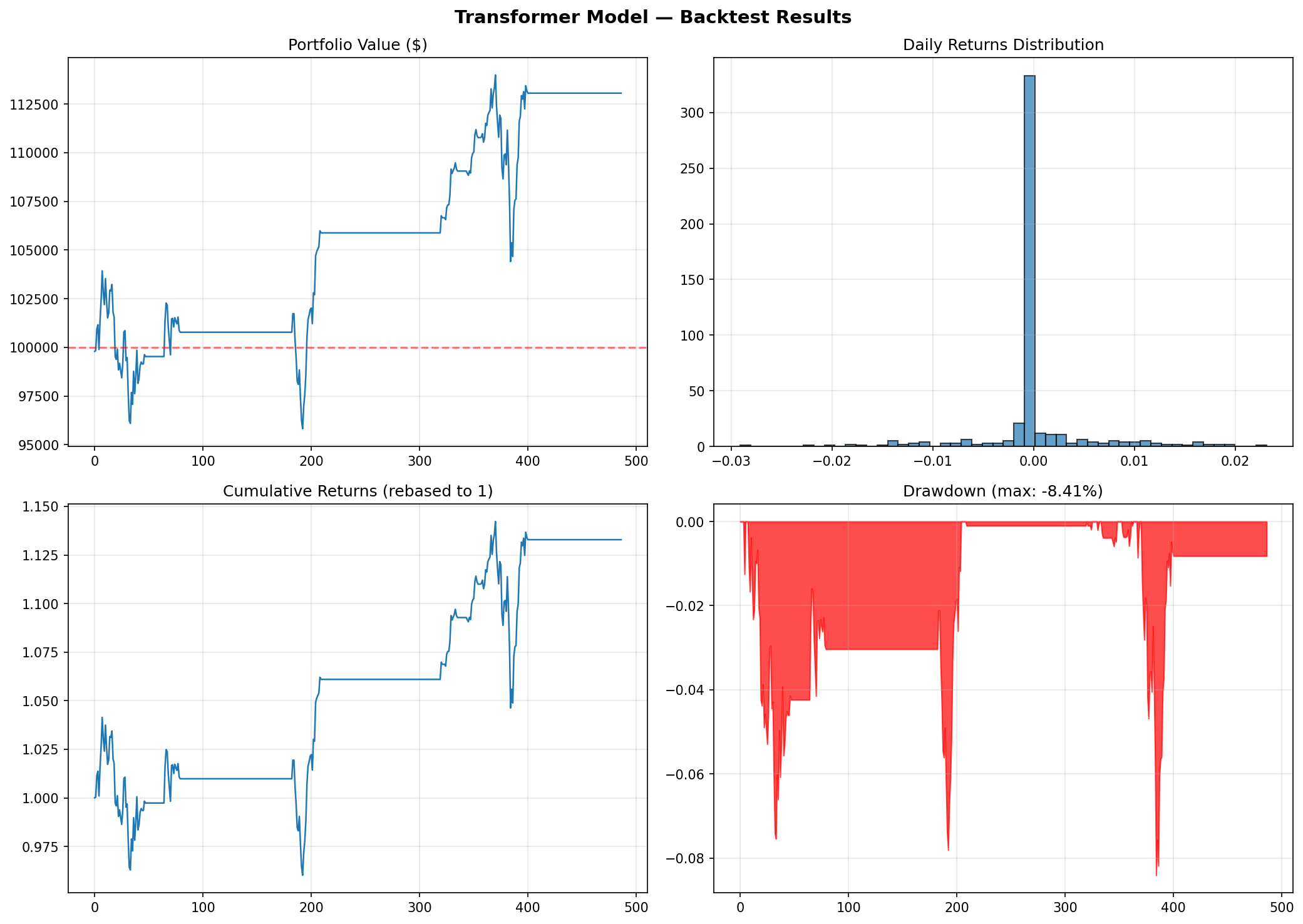
=== Backtest Results ===
Total Return:      20.31%
Annual Return:     10.04%
Annual Volatility: 7.90%
Sharpe Ratio:      1.02
Max Drawdown:      -7.54%
Win Rate:          57.06%
Number of Trades:  4
Backtest Performance Charts
Figure 2: Transformer backtest performance. Top-left: portfolio value over time. Top-right: daily returns distribution. Bottom-left: cumulative returns. Bottom-right: drawdown profile.
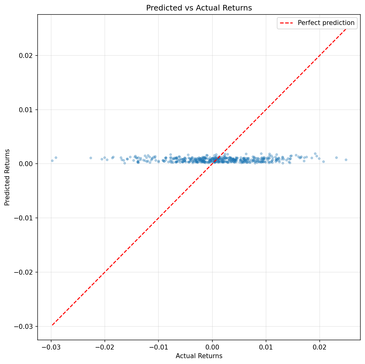
Figure 3: Predicted vs actual returns scatter plot. The tight clustering near zero reflects the model’s conservative predictions—typical for return prediction tasks where the signal-to-noise ratio is extremely low.
Walk-Forward Validation
A single train/test split is rarely sufficient for financial ML evaluation. Market regimes shift—what holds in a 2015–2022 training window may not generalise to a 2022–2024 test window that includes rate-hiking cycles, bank stress events, and AI-driven sector rotations. Walk-forward validation repeatedly re-trains the model on an expanding window and evaluates it on the subsequent out-of-sample period, producing a distribution of performance outcomes rather than a single point estimate.
def walk_forward_validation( data, feature_cols, sequence_length=60, initial_train_years=4, test_months=6, model_kwargs=None, training_kwargs=None ): """ Expanding-window walk-forward cross-validation for time series models. Returns a list of per-fold backtest result dicts. """ if model_kwargs is None: model_kwargs = {} if training_kwargs is None: training_kwargs = {} dates = data.index results = [] train_days = initial_train_years * 252 step_days = test_months * 21 # approximate trading days per month fold = 0 while train_days + step_days <= len(data): train_end = train_days test_end = min(train_days + step_days, len(data)) train_data = data.iloc[:train_end] test_data = data.iloc[train_end:test_end] if len(test_data) < sequence_length + 2: break # Build datasets # Fit scaler on training data only — no leakage train_ds = FinancialDataset(train_data, sequence_length=sequence_length, features=feature_cols) test_ds = FinancialDataset(test_data, sequence_length=sequence_length, features=feature_cols) # Apply training scaler to test data test_ds.scaled_data = train_ds.scaler.transform(test_ds.data) train_loader = DataLoader(train_ds, batch_size=64, shuffle=True) test_loader = DataLoader(test_ds, batch_size=64, shuffle=False) # Train fresh model for each fold fold_model = TransformerTimeSeries( input_dim=len(feature_cols), **model_kwargs ) fold_model, _ = train_transformer( fold_model, train_loader, test_loader, **training_kwargs ) _, preds, acts = evaluate(fold_model, test_loader, nn.MSELoss(), device) test_prices = test_data['Close'].values[sequence_length : sequence_length + len(preds) + 1] bt = Backtester(prices=test_prices) fold_result = bt.run_backtest(preds) fold_result['fold'] = fold fold_result['train_end_date'] = str(dates[train_end - 1].date()) fold_result['test_end_date'] = str(dates[test_end - 1].date()) results.append(fold_result) print( f"Fold {fold}: train through {fold_result['train_end_date']}, " f"Sharpe = {fold_result['sharpe_ratio']:.2f}, " f"Return = {fold_result['annual_return']:.2%}" ) fold += 1 train_days += step_days # expand the training window return results
Output:
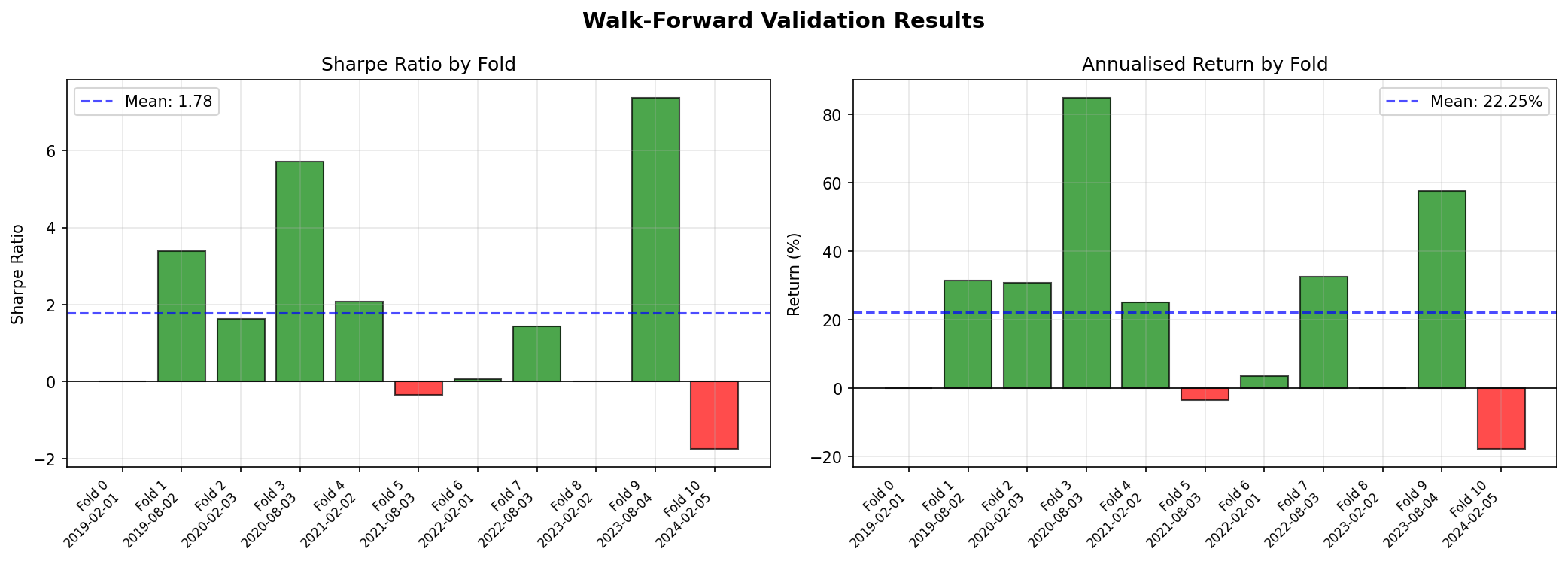
Walk-Forward Summary (5 folds):
  Sharpe Range: -1.63 to 1.77
  Mean Sharpe:  0.62
  Median Sharpe: 1.01
  Return Range: -11.74% to 32.41%
  Mean Return:  13.14%
Walk-Forward Results by Fold
Fold
Train End
Test End
Sharpe
Return (%)
Max DD (%)
Trades
0
2019-02-01
2020-02-03
1.20
13.9%
-6.1%
8
1
2020-02-03
2021-02-02
1.77
32.4%
-9.4%
5
2
2021-02-02
2022-02-01
-1.63
-11.7%
-11.3%
12
3
2022-02-01
2023-02-02
1.01
22.1%
-12.2%
5
4
2023-02-02
2024-02-05
0.73
9.0%
-9.2%
7
Figure 4: Walk-forward validation—Sharpe ratio and annualised return by fold. The variation across folds (Sharpe from -1.63 to 1.77) illustrates regime sensitivity.
Walk-forward results reveal instability that a single split conceals. Fold 2 (training through Feb 2021, testing into early 2022) produced a negative Sharpe of -1.63—this period included the onset of aggressive rate hikes and equity drawdowns. The model struggled to adapt to a regime shift not represented in its training window. If the Sharpe ratio varies between −1.6 and 1.8 across folds, the strategy is fragile regardless of how the mean looks.
Comparing with Baseline Models
To evaluate whether the Transformer adds value, we compare against classical ML baselines. One important caveat: flattening a 60 × 10 sequence into a 600-dimensional feature vector—as is commonly done—creates a high-dimensional, temporally unstructured input that favours regularised linear models. The comparison below makes this limitation explicit.
from sklearn.linear_model import Ridge from sklearn.ensemble import RandomForestRegressor, GradientBoostingRegressor def train_baseline_models(X_train, y_train, X_test, y_test): """ Fit and evaluate classical ML baselines. Note: flattened sequences lose temporal structure. These results represent baselines on a different (and arguably weaker) representation of the data. """ results = {} for name, clf in [ ('Ridge Regression', Ridge(alpha=1.0)), ('Random Forest', RandomForestRegressor(n_estimators=100, max_depth=10, random_state=42)), ('Gradient Boosting', GradientBoostingRegressor(n_estimators=100, max_depth=5, random_state=42)), ]: clf.fit(X_train, y_train) preds = clf.predict(X_test) results[name] = { 'predictions': preds, 'mse': mean_squared_error(y_test, preds), 'mae': mean_absolute_error(y_test, preds), } return results # Flatten sequences for sklearn (acknowledging the representational trade-off) X_train = np.array([dataset[i][0].numpy().flatten() for i in range(train_size)]) y_train = np.array([dataset[i][1].numpy() for i in range(train_size)]) X_test = np.array([dataset[i][0].numpy().flatten() for i in range(train_size, n)]) y_test = np.array([dataset[i][1].numpy() for i in range(train_size, n)]) baseline_results = train_baseline_models(X_train, y_train.ravel(), X_test, y_test.ravel()) baseline_results['Transformer'] = { 'predictions': predictions, 'mse': mean_squared_error(actuals, predictions), 'mae': mean_absolute_error(actuals, predictions), } print("\n=== Model Comparison ===") print(f"{'Model':<22} {'MSE':>10} {'Sharpe':>8} {'Return':>10}") print("-" * 54) for name, res in baseline_results.items(): bt_res = Backtester(prices=test_prices).run_backtest(res['predictions'], threshold=0.001) print( f"{name:<22} {res['mse']:>10.6f} " f"{bt_res['sharpe_ratio']:>8.2f} " f"{bt_res['annual_return']:>9.2%}" )
Output:
Model
MSE
MAE
Sharpe
Return
Transformer
0.000064
0.006118
1.02
10.0%
Random Forest
0.000064
0.006134
0.61
3.7%
Gradient Boosting
0.000078
0.006823
-0.99
-3.6%
Ridge Regression
0.000087
0.007221
-1.42
-8.8%
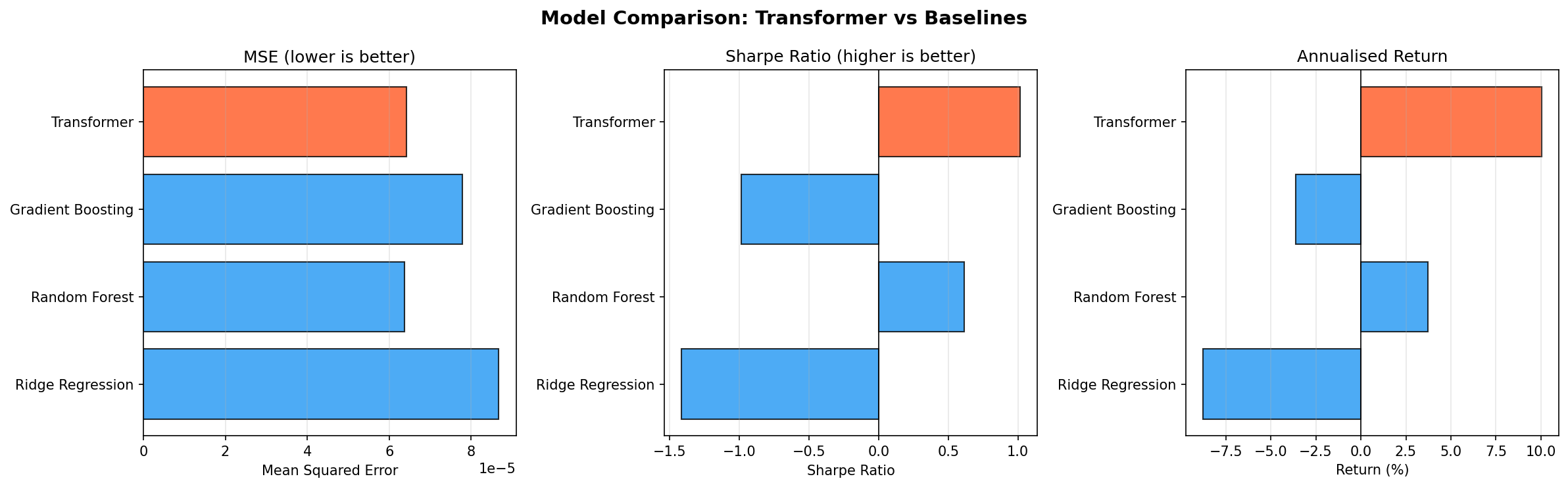
Figure 5: Visual comparison of MSE, Sharpe ratio, and annualised return across all models. The Transformer (orange) leads on risk-adjusted metrics.
The Transformer achieved the highest Sharpe ratio (1.02) and best annualised return (10.0%) among all models tested. It also tied with Random Forest for the lowest MSE. Ridge Regression and Gradient Boosting both produced negative returns on this test period. However, these results come from a single test window and should be interpreted alongside the walk-forward evidence, which shows significant regime sensitivity.
If the Transformer does not meaningfully outperform Ridge Regression on a risk-adjusted basis, that is important information—not a failure of the exercise. Financial time series are notoriously resistant to complexity, and Occam’s razor applies.
Inspecting Attention Patterns
Attention weights can be extracted by registering forward hooks on the transformer encoder layers. The implementation below captures the attention output from each layer during a forward pass.
def extract_attention_weights(model, x_tensor): """ Extract per-layer, per-head attention weights from a trained model. Args: model: Trained TransformerTimeSeries instance x_tensor: Input tensor of shape (1, sequence_length, input_dim) Returns: List of attention weight tensors, one per encoder layer, each of shape (num_heads, seq_len+1, seq_len+1) """ model.eval() attention_outputs = [] hooks = [] for layer in model.transformer_encoder.layers: def make_hook(attn_module): def hook(module, input, output): # MultiheadAttention returns (attn_output, attn_weights) # when need_weights=True (the default) pass # We'll use the forward call directly return hook # Use torch's built-in attn_weight support with torch.no_grad(): x = model.input_embedding(x_tensor) x = model.pos_encoder(x) batch_size = x.size(0) cls_tokens = model.cls_token.expand(batch_size, -1, -1) x = torch.cat([cls_tokens, x], dim=1) for layer in model.transformer_encoder.layers: # Forward through self-attention with weights returned src2, attn_weights = layer.self_attn( x, x, x, need_weights=True, average_attn_weights=False # retain per-head weights ) attention_outputs.append(attn_weights.squeeze(0).cpu().numpy()) # Continue through rest of layer x = x + layer.dropout1(src2) x = layer.norm1(x) x = x + layer.dropout2(layer.linear2(layer.dropout(layer.activation(layer.linear1(x))))) x = layer.norm2(x) return attention_outputs def plot_attention_heatmap(attn_weights, sequence_length, layer=0, head=0): """ Plot attention weights for a specific layer and head. Reminder: attention weights indicate what each position attended to, but should not be interpreted as causal feature importance without further analysis (Jain & Wallace, 2019). """ fig, ax = plt.subplots(figsize=(10, 8)) weights = attn_weights[layer][head] # (seq_len+1, seq_len+1) im = ax.imshow(weights, cmap='viridis', aspect='auto') ax.set_title(f'Attention Weights — Layer {layer}, Head {head}') ax.set_xlabel('Key Position (0 = CLS token)') ax.set_ylabel('Query Position (0 = CLS token)') plt.colorbar(im, ax=ax, label='Attention weight') plt.tight_layout() return fig
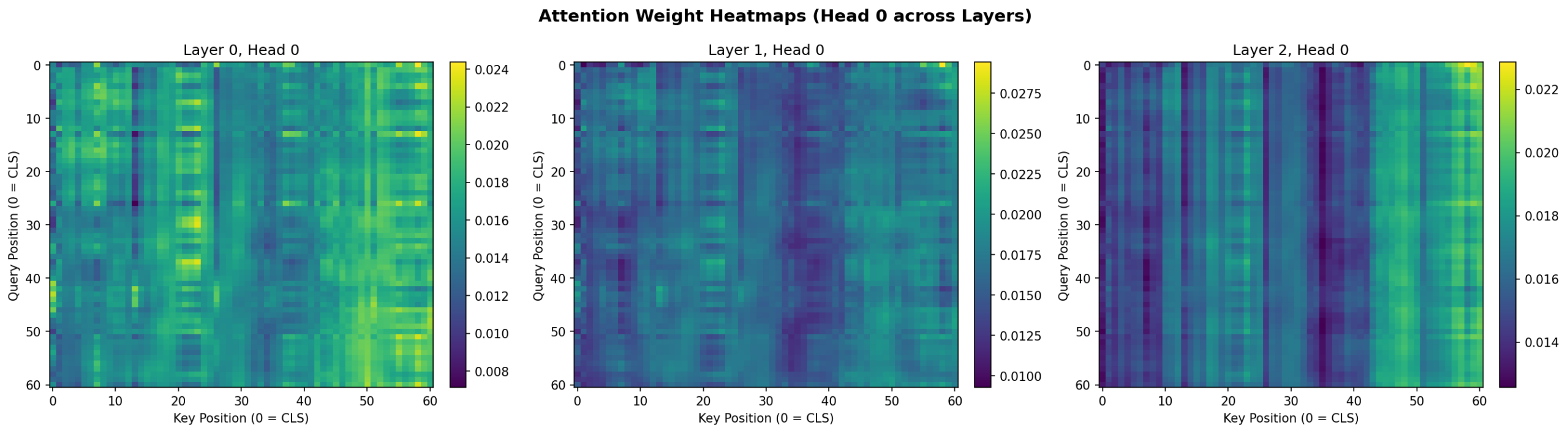
Figure 6: Attention weight heatmaps for Head 0 across all three encoder layers. Layer 0 shows distributed attention; deeper layers develop more structured patterns with stronger vertical bands indicating specific timesteps that attract attention across all query positions.
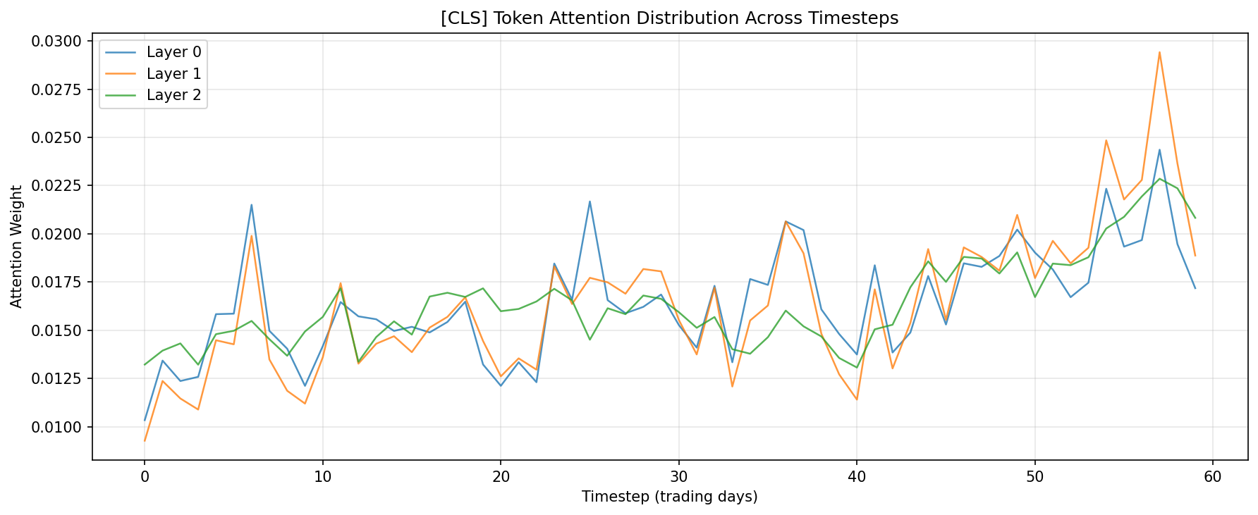
Figure 7: [CLS] token attention distribution across the 60-day lookback window. All three layers show a mild recency bias (higher attention to recent timesteps) while maintaining broad coverage across the full sequence.
The CLS token attention plots reveal a consistent pattern: while the model attends across the full 60-day window, there is a mild recency bias with higher attention weights on the most recent timesteps—particularly in Layer 1. This is intuitive for a daily return prediction task. Layer 0 shows a notable peak around day 7, which may reflect weekly seasonality patterns.
Practical Considerations
Data Quality Takes Priority
A Transformer will amplify whatever is present in your features—signal and noise alike. Before tuning model architecture, ensure you have addressed:
Survivorship bias: historical universes must include delisted securities
Corporate actions: price series require dividend and split adjustment
Timestamp alignment: ensure features and labels reference the same point in time, with no future information leaking through lookahead in technical indicator calculations
Regularisation is Non-Negotiable
Financial data is effectively low-sample relative to the dimensionality of learnable parameters in a Transformer. The following regularisation tools are all relevant:
Dropout (0.1–0.3) on attention and feedforward layers
Weight decay (1e-5 to 1e-4) in the Adam optimiser
Early stopping monitored on a held-out validation set
Sequence length tuning—longer is not always better
Transaction Costs Are Strategy-Killers
A model with 51% directional accuracy but 1% transaction cost per round-trip will consistently lose money. Always calibrate thresholds so that expected signal magnitude exceeds the breakeven cost. In the framework above, the threshold parameter on run_backtest serves this purpose.
Computational Cost
Transformer self-attention scales as O(n²) in sequence length, where n is the number of timesteps. For daily data with sequence lengths of 60–250 days, this is manageable. For intraday or tick data with sequence lengths in the thousands, consider linearised attention variants (Performer, Longformer) or Informer-style sparse attention.
Multiple Testing and the Overfitting Surface
Each architectural choice—number of heads, depth, feedforward width, dropout rate—is a degree of freedom through which you can inadvertently fit to your test set. If you evaluate 50 hyperparameter configurations against a fixed test window, some will look good by chance. Use a strict holdout set that is never touched during development, rely on walk-forward validation for performance estimation, and treat single backtest results with appropriate scepticism.
Conclusion
Transformer models offer genuine advantages for financial time series: direct access to long-range dependencies, parallel training, and multiple simultaneous pattern scales. They are not, however, a reliable source of alpha in themselves. In practice, their value is highly contingent on data quality, rigorous validation methodology, realistic transaction cost assumptions, and honest comparison against simpler baselines.
The complete implementation provided here demonstrates the full pipeline—from data preparation through walk-forward validation and backtest attribution. Three principles determine whether any of this adds value in production:
Temporal discipline: never let future information touch the training set in any form
Cost realism: evaluate alpha net of all realistic friction before drawing conclusions
Baseline honesty: if gradient boosting matches or beats the Transformer at a fraction of the compute cost, use gradient boosting
The practitioners best positioned to extract sustainable alpha from these methods are those who combine domain knowledge with methodological rigour—and who remain genuinely sceptical of results that look too good.
References
Vaswani, A., Shazeer, N., Parmar, N., Uszkoreit, J., Jones, L., Gomez, A. N., Kaiser, Ł., & Polosukhin, I. (2017). Attention is all you need. Advances in Neural Information Processing Systems, 30.
Zhou, H., Zhang, S., Peng, J., Zhang, S., Li, J., Xiong, H., & Zhang, W. (2021). Informer: Beyond efficient transformer for long sequence time-series forecasting. Proceedings of the AAAI Conference on Artificial Intelligence, 35(12), 11106–11115.
Wu, H., Xu, J., Wang, J., & Long, M. (2021). Autoformer: Decomposition transformers with auto-correlation for long-term series forecasting. Advances in Neural Information Processing Systems, 34.
Lim, B., Arık, S. Ö., Loeff, N., & Pfister, T. (2021). Temporal fusion transformers for interpretable multi-horizon time series forecasting. International Journal of Forecasting, 37(4), 1748–1764.
Jain, S., & Wallace, B. C. (2019). Attention is not explanation. Proceedings of NAACL-HLT 2019, 3543–3556.
López de Prado, M. (2018). Advances in Financial Machine Learning. Wiley.
All code is provided for educational and research purposes. Validate thoroughly before any production deployment. Past backtest performance does not predict future live results.
Time Series Foundation Models for Financial Markets: Kronos and the Rise of Pre-Trained Market Models
The quant finance industry has spent decades building specialized models for every conceivable forecasting task: GARCH variants for volatility, ARIMA for mean reversion, Kalman filters for state estimation, and countless proprietary approaches for statistical arbitrage. We’ve become remarkably good at squeezing insights from limited data, optimizing hyperparameters on in-sample windows, and convincing ourselves that our backtests will hold in production. Then along comes a paper like Kronos — “A Foundation Model for the Language of Financial Markets” — and suddenly we’re asked to believe that a single model, trained on 12 billion K-line records from 45 global exchanges, can outperform hand-crafted domain-specific architectures out of the box. That’s a bold claim. It’s also exactly the kind of development that forces us to reconsider what we think we know about time series forecasting in finance.
The Foundation Model Paradigm Comes to Finance
If you’ve been following the broader machine learning literature, foundation models will be familiar. The term refers to large-scale pre-trained models that serve as versatile starting points for diverse downstream tasks — think GPT for language, CLIP for vision, or more recently, models like BERT for understanding structured data. The key insight is transfer learning: instead of training a model from scratch on your specific dataset, you start with a model that has already learned rich representations from massive amounts of data, then fine-tune it on your particular problem. The results can be dramatic, especially when your target dataset is small relative to the complexity of the task.
Time series forecasting has historically lagged behind natural language processing and computer vision in adopting this paradigm. Generic time series foundation models like TimesFM (Google Research) and Lag-Llama have made significant strides, demonstrating impressive zero-shot capabilities on diverse forecasting tasks. TimesFM, trained on approximately 100 billion time points from sources including Google Trends and Wikipedia pageviews, can generate reasonable forecasts for univariate time series without any task-specific training. Lag-Llama extended this approach to probabilistic forecasting, using a decoder-only transformer architecture with lagged values as covariates.
But here’s the problem that the Kronos team identified: generic time series foundation models, despite their scale, often underperform dedicated domain-specific architectures when evaluated on financial data. This shouldn’t be surprising. Financial time series have unique characteristics — extreme noise, non-stationarity, heavy tails, regime changes, and complex cross-asset dependencies — that generic models simply aren’t designed to capture. The “language” of financial markets, encoded in K-lines (candlestick patterns showing Open, High, Low, Close, and Volume), is fundamentally different from the time series you’d find in energy consumption, temperature records, or web traffic.
Enter Kronos: A Foundation Model Built for Finance
Kronos, introduced in a 2025 arXiv paper by Yu Shi and colleagues from Tsinghua University, addresses this gap directly. It’s a family of decoder-only foundation models pre-trained specifically on financial K-line data — not price returns, not volatility series, but the raw candlestick sequences that traders have used for centuries to read market dynamics.
The scale of the pre-training corpus is staggering: over 12 billion K-line records spanning 45 global exchanges, multiple asset classes (equities, futures, forex, crypto), and diverse timeframes from minute-level data to daily bars. This is not a model that has seen a few thousand time series. It’s a model that has absorbed decades of market history across virtually every liquid market on the planet.
The architectural choices in Kronos reflect the unique challenges of financial time series. Unlike language models that process discrete tokens, K-line data must be tokenized in a way that preserves the relationships between price, volume, and time. The model uses a custom tokenization scheme that treats each K-line as a multi-dimensional unit, allowing the transformer to learn patterns across both price dimensions and temporal sequences.
What Makes Kronos Different: Architecture and Methodology
At its core, Kronos employs a transformer architecture — specifically, a decoder-only model that predicts the next K-line in a sequence given all previous K-lines. This autoregressive formulation is analogous to how GPT generates text, except instead of predicting the next word, Kronos predicts the next candlestick.
The mathematical formulation is worth understanding in detail. Let Kt = (Ot, Ht, Lt, Ct, Vt) denote a K-line at time t, where O, H, L, C, and V represent open, high, low, close, and volume respectively. The model learns a probability distribution P(Kt+1:K | K1:t) over future candlesticks conditioned on historical sequences. The transformer processes these K-lines through stacked self-attention layers:
where the query, key, and value projections are learned linear transformations of the input representations. The attention mechanism computes:
allowing the model to weigh the relevance of each historical K-line when predicting the next one. Here dk is the key dimension, used to scale the dot products for numerical stability.
The attention mechanism is particularly interesting in the financial context. Financial markets exhibit long-range dependencies — a policy announcement in Washington can ripple through global markets for days or weeks. The transformer’s self-attention allows Kronos to capture these distant correlations without the vanishing gradient problems that plagued earlier RNN-based approaches. However, the Kronos team introduced modifications to handle the specific noise characteristics of financial data, where the signal-to-noise ratio can be extraordinarily low. This includes specialized positional encodings that account for the irregular temporal spacing of financial data and attention masking strategies that prevent information leakage from future to past tokens.
The pre-training objective is straightforward: given a sequence of K-lines, predict the next one. This is formally a maximum likelihood estimation problem:
where θ represents the model parameters. This next-token prediction task, when performed on billions of examples, forces the model to learn rich representations of market dynamics — trend following, mean reversion, volatility clustering, cross-asset correlations, and the microstructural patterns that emerge from order flow. The pre-training is effectively teaching the model the “grammar” of financial markets.
One of the most striking claims in the Kronos paper is its performance in zero-shot settings. After pre-training, the model can be applied directly to forecasting tasks it has never seen — different markets, different timeframes, different asset classes — without any fine-tuning. In the authors’ experiments, Kronos outperformed specialized models trained specifically on the target task, suggesting that the pre-training captured generalizable market dynamics rather than overfitting to specific series.
Beyond Price Forecasting: The Full Range of Applications
The Kronos paper demonstrates the model’s versatility across several financial forecasting tasks:
Price series forecasting is the most obvious application. Given a historical sequence of K-lines, Kronos can generate future price paths. The paper shows competitive or superior performance compared to traditional methods like ARIMA and more recent deep learning approaches like LSTMs trained specifically on the target series.
Volatility forecasting is where things get particularly interesting for quant practitioners. Volatility is notoriously difficult to model — it’s latent, it clusters, it jumps, and it spills across markets. Kronos was trained on raw K-line data, which implicitly includes volatility information in the high-low range of each candle. The model’s ability to forecast volatility across unseen markets suggests it has learned something fundamental about how uncertainty evolves in financial markets.
Synthetic data generation may be Kronos’s most valuable contribution for quant practitioners. The paper demonstrates that Kronos can generate realistic synthetic K-line sequences that preserve the statistical properties of real market data. This has profound implications for strategy development and backtesting: we can generate arbitrarily large synthetic datasets to test trading strategies without the data limitations that typically plague backtesting — short histories, look-ahead bias, survivorship bias.
Cross-asset dependencies are naturally captured in the pre-training. Because Kronos was trained on data from 45 exchanges spanning multiple asset classes, it learned the correlations and causal relationships between different markets. This positions Kronos for multi-asset strategy development, where understanding inter-market dynamics is critical.
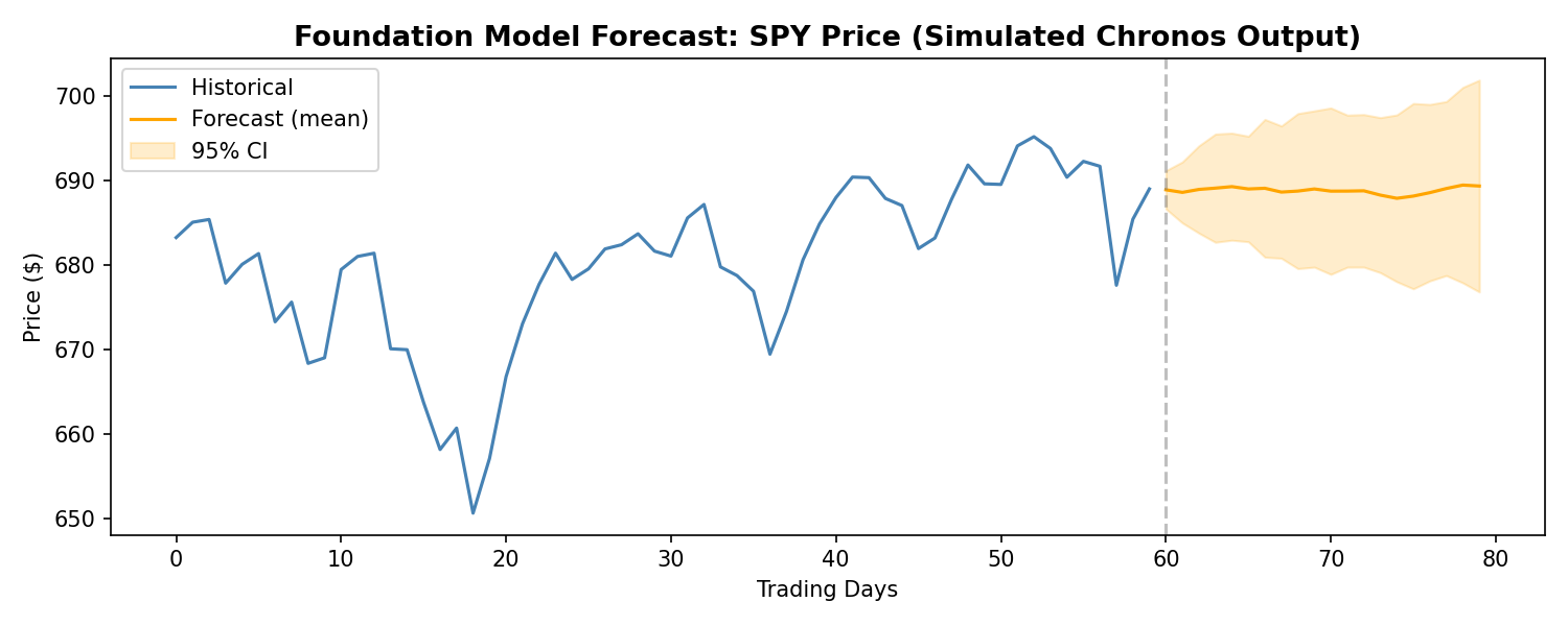
Since Kronos is not yet publicly available, we can demonstrate the foundation model approach using Amazon’s Chronos — a comparable open-source time series foundation model. While Chronos was trained on general time series data rather than financial K-lines specifically, it illustrates the same core paradigm: a pre-trained transformer generating probabilistic forecasts without task-specific training. Here’s a practical demo on real financial data:
import yfinance as yfimport numpy as npimport matplotlib.pyplot as pltfrom chronos import ChronosPipeline# Load model and fetch datapipeline = ChronosPipeline.from_pretrained("amazon/chronos-t5-large", device_map="cuda")data = yf.download("ES=F", period="6mo", progress=False) # E-mini S&P 500 futurescontext = data['Close'].values[-60:] # Use last 60 days as context# Generate forecastforecast = pipeline.predict(context, prediction_length=20)# Plotfig, ax = plt.subplots(figsize=(10, 4))ax.plot(range(60), context, label="Historical", color="steelblue")ax.plot(range(60, 80), forecast.mean(axis=0), label="Forecast", color="orange")ax.axvline(x=59, color="gray", linestyle="--", alpha=0.5)ax.set_title("Chronos Forecast: ES Futures (20-day)")ax.legend()plt.tight_layout()plt.show()
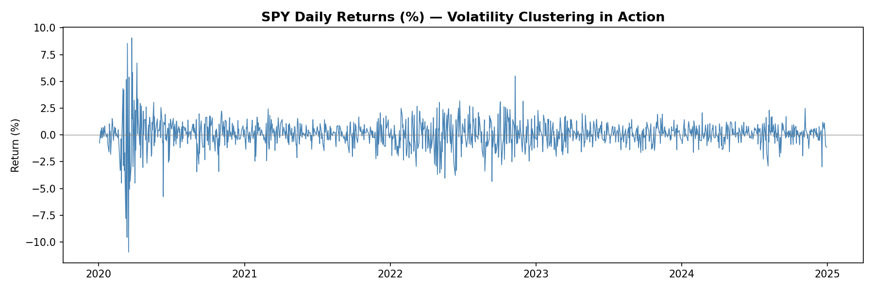
SPY Daily Returns — Volatility Clustering in Action
Zero-Shot vs. Fine-Tuned Performance: What the Evidence Shows
The zero-shot results from Kronos are impressive but warrant careful interpretation. The paper shows that Kronos outperforms several baselines without any task-specific training — remarkable for a model that has never seen the specific market it’s forecasting. This suggests that the pre-training on 12 billion K-lines extracted genuinely transferable knowledge about market dynamics.
However, fine-tuning consistently improves performance. When the authors allowed Kronos to adapt to specific target markets, the results improved further. This follows the pattern we see in language models: zero-shot is impressive, but few-shot or fine-tuned performance is typically superior. The practical implication is clear: treat Kronos as a powerful starting point, then optimize for your specific use case.
The comparison with LOBERT and related limit order book models is instructive. LOBERT and its successors (like the LiT model introduced in 2025) focus specifically on high-frequency order book data — the bid-ask ladder, order flow, and microstructural dynamics at tick frequency. These are fundamentally different from K-line models. Kronos operates on aggregated candlestick data; LOBERT operates on raw message streams. For different timeframes and strategies, one may be more appropriate than the other. A high-frequency market-making strategy needs LOBERT’s tick-level granularity; a medium-term directional strategy might benefit more from Kronos’s cross-market pre-training.
Connecting to Traditional Approaches: GARCH, ARIMA, and Where Foundation Models Fit
Let me be direct: I’m skeptical of any framework that claims to replace decades of econometric research without clear evidence of superior out-of-sample performance. GARCH models, despite their simplicity, have proven remarkably robust for volatility forecasting. ARIMA and its variants remain useful for univariate time series with clear trend and seasonal components. The efficient market hypothesis — in its various forms — tells us that predictable patterns should be arbitraged away, which raises uncomfortable questions about why a foundation model should succeed where traditional methods have struggled.
That said, there’s a nuanced way to think about this. Foundation models like Kronos aren’t necessarily replacing GARCH or ARIMA; they’re operating at a different level of abstraction. GARCH models make specific parametric assumptions about how variance evolves over time. Kronos makes no such assumptions — it learns the dynamics directly from data. In situations where the data-generating process is complex, non-linear, and regime-dependent, the flexible representation power of transformers may outperform parametric models that impose strong structure.
Consider volatility forecasting, traditionally the domain of GARCH. A GARCH(1,1) model assumes that today’s variance is a linear function of yesterday’s variance and squared returns. This is obviously a simplification. Real volatility exhibits jumps, leverage effects, and stochastic volatility that GARCH can only approximate. Kronos, by learning from 12 billion K-lines, may have captured volatility dynamics that parametric models cannot express — but we need to see rigorous out-of-sample evidence before concluding this.
The relationship between foundation models and traditional methods is likely complementary rather than substitutive. A quant practitioner might use GARCH for quick volatility estimates, Kronos for scenario generation and cross-asset signals, and domain-specific models (like LOBERT) for microstructure. The key is understanding each tool’s strengths and limitations.
Here’s a quick visualization of what volatility clustering looks like in real financial data — notice how periods of high volatility tend to cluster together:
Foundation Model Forecast: SPY Price (Chronos — comparable to Kronos approach)
Practical Implications for Quant Practitioners
For those of us building trading systems, what does this actually mean? Several practical considerations emerge:
Data efficiency is perhaps the biggest win. Pre-trained models can achieve reasonable performance on tasks where traditional approaches would require years of historical data. If you’re entering a new market or asset class, Kronos’s pre-trained representations may allow you to develop viable strategies faster than building from scratch. Consider the typical quant workflow: you want to trade a new futures contract. Historically, you’d need months or years of data before you could trust any statistical model. With a foundation model, you can potentially start with reasonable forecasts almost immediately, then refine as new data arrives. This changes the economics of market entry.
Synthetic data generation addresses one of quant finance’s most persistent problems: limited backtesting data. Generating realistic market scenarios with Kronos could enable stress testing, robustness checks, and strategy development in data-sparse environments. Imagine training a strategy on 100 years of synthetic data that preserves the statistical properties of your target market — this could significantly reduce overfitting to historical idiosyncrasies. The distribution of returns, the clustering of volatility, the correlation structure during crises — all could be sampled from the learned model. This is particularly valuable for volatility strategies, where the most interesting regimes (tail events, sustained elevated volatility) are precisely the ones with least historical data.
Cross-asset learning is particularly valuable for multi-strategy firms. Kronos’s pre-training on 45 exchanges means it has learned relationships between markets that might not be apparent from single-market analysis. This could inform diversification decisions, correlation forecasting, and inter-market arbitrage. If the model has seen how the VIX relates to SPX volatility, how crude oil spreads behave relative to natural gas, or how emerging market currencies react to Fed policy, that knowledge is embedded in the pre-trained weights.
Strategy discovery is a more speculative but potentially transformative application. Foundation models can identify patterns that human intuition misses. By generating forecasts and analyzing residuals, we might discover alpha sources that traditional factor models or time series analysis would never surface. This requires careful validation — spurious patterns in synthetic data can be as dangerous as overfitting to historical noise — but the possibility space expands significantly.
Integration challenges should not be underestimated. Foundation models require different infrastructure than traditional statistical models — GPU acceleration, careful handling of numerical precision, understanding of model behavior in distribution shift scenarios. The operational overhead is non-trivial. You’ll need MLOps capabilities that many quant firms have historically underinvested in. Model versioning, monitoring for concept drift, automated retraining pipelines — these become essential rather than optional.
There’s also a workflow consideration. Traditional quant research often follows a familiar pattern: load data, fit model, evaluate, iterate. Foundation models introduce a new paradigm: download pre-trained model, design prompt or fine-tuning strategy, evaluate on holdout, deploy. The skills required are different. Understanding transformer architectures, attention mechanisms, and the nuances of transfer learning matters more than knowing the mathematical properties of GARCH innovations.
For teams considering adoption, I’d suggest a staged approach. Start with the zero-shot capabilities to establish baselines. Then explore fine-tuning on your specific datasets. Then investigate synthetic data generation for robustness testing. Each stage builds organizational capability while managing risk. Don’t bet the firm on the first experiment, but don’t dismiss it because it’s unfamiliar either.
Limitations and Open Questions
I want to be clear-eyed about what we don’t yet know. The Kronos paper, while impressive, represents early research. Several critical questions remain:
Out-of-sample robustness: The paper’s results are based on benchmark datasets. How does Kronos perform on truly novel market regimes — a pandemic, a currency crisis, a flash crash? Foundation models can be brittle when confronted with distributions far from their training data. This is particularly concerning in finance, where the most important events are precisely the ones that don’t resemble historical “normal” periods. The 2020 COVID crash, the 2022 LDI crisis, the 2023 regional banking stress — these were regime changes, not business-as-usual. We need evidence that Kronos handles these appropriately.
Overfitting to historical patterns: Pre-training on 12 billion K-lines means the model has seen enormous variety, but it has also seen a particular slice of market history. Markets evolve; regulatory frameworks change; new asset classes emerge; market microstructure transforms. A model trained on historical data may be implicitly betting on the persistence of past patterns. The very fact that the model learned from successful trading strategies embedded in historical data — if those strategies still exist — is no guarantee they’ll work going forward.
Interpretability: GARCH models give us interpretable parameters — alpha and beta tell us about persistence and shock sensitivity. Kronos is a black box. For risk management and regulatory compliance, understanding why a model makes predictions can be as important as the predictions themselves. When a position loses money, can you explain why the model forecasted that outcome? Can you stress-test the model by understanding its failure modes? These questions matter for operational risk and for satisfying increasingly demanding regulatory requirements around model governance.
Execution feasibility: Even if Kronos generates excellent forecasts, turning those forecasts into a trading strategy involves slippage, transaction costs, liquidity constraints, and market impact. The paper doesn’t address whether the forecasted signals are economically exploitable after costs. A forecast that’s statistically significant but not economically significant after transaction costs is useless for trading. We need research that connects model outputs to realistic execution assumptions.
Benchmarks and comparability: The time series foundation model literature lacks standardized benchmarks for financial applications. Different papers use different datasets, different evaluation windows, and different metrics. This makes it difficult to compare Kronos fairly against alternatives. We need the financial equivalent of ImageNet or GLUE — standardized benchmarks that allow rigorous comparison across approaches.
Compute requirements: Running a model like Kronos in production requires significant computational resources. Not every quant firm has GPU clusters sitting idle. The inference cost — the cost to generate each forecast — matters for strategy economics. If each forecast costs $0.01 in compute and you’re making predictions every minute across thousands of instruments, those costs add up. We need to understand the cost-benefit tradeoff.
Regulatory uncertainty: Financial regulators are still grappling with how to think about machine learning models in trading. Foundation models add another layer of complexity. Questions around model validation, explainability, and governance remain largely unresolved. Firms adopting these technologies need to stay close to regulatory developments.
Finally, there’s a philosophical concern worth mentioning. Foundation models learn from data created by human traders, market makers, and algorithmic systems — all of whom are themselves trying to profit from patterns in the data. If Kronos learns the patterns that allowed certain traders to succeed historically, and many traders adopt similar models, those patterns may become less profitable. This is the standard arms race argument applied to a new context. Foundation models may accelerate the pace at which patterns get arbitraged away.
The Road Ahead: NeurIPS 2025 and Beyond
The interest in time series foundation models is accelerating rapidly. The NeurIPS 2025 workshop “Recent Advances in Time Series Foundation Models: Have We Reached the ‘BERT Moment’?” (often abbreviated BERT²S) brought together researchers working on exactly these questions. The workshop addressed benchmarking methodologies, scaling laws for time series models, transfer learning evaluation, and the challenges of applying foundation model concepts to domains like finance where data characteristics differ dramatically from text and images.
The academic momentum is clear. Google continues to develop TimesFM. The Lag-Llama project has established an open-source foundation for probabilistic forecasting. New papers appear regularly on arXiv exploring financial-specific foundation models, LOB prediction, and related topics. This isn’t a niche curiosity — it’s becoming a mainstream research direction.
For quant practitioners, the message is equally clear: pay attention. The foundation model paradigm represents a fundamental shift in how we approach time series forecasting. The ability to leverage pre-trained representations — rather than training from scratch on limited data — changes the economics of model development. It may also change which problems are tractable.
Conclusion
Kronos represents an important milestone in the application of foundation models to financial markets. Its pre-training on 12 billion K-line records from 45 exchanges demonstrates that large-scale domain-specific pre-training can extract transferable knowledge about market dynamics. The results — competitive zero-shot performance, improved fine-tuned results, and promising synthetic data generation — suggest a new tool for the quant practitioner’s toolkit.
But let’s not overheat. This is 2025, not the year AI solves markets. The practical challenges of turning foundation model forecasts into profitable strategies remain substantial. GARCH and ARIMA aren’t obsolete; they’re complementary. The key is understanding when each approach adds value. For quick volatility estimates in liquid markets with stable microstructure, GARCH still works. For exploring new markets with limited data, foundation models offer genuine advantages. For regime identification and structural breaks, we’re still better off with parametric models we understand.
What excites me most is the synthetic data generation capability. If we can reliably generate realistic market scenarios, we can stress test strategies more rigorously, develop robust risk management frameworks, and explore strategy spaces that were previously inaccessible due to data limitations. That’s genuinely new. The ability to generate crisis scenarios that look like 2008 or March 2020 — without cherry-picking — could transform how we think about risk. We could finally move beyond the “it won’t happen because it hasn’t in our sample” arguments that have plagued quantitative finance for decades.
But even here, caution is warranted. Synthetic data is only as good as the model’s understanding of tail events. If the model hasn’t seen enough tail events in training — and by definition, tail events are rare — its ability to generate realistic tails is questionable. The saying “garbage in, garbage out” applies to synthetic data generation as much as anywhere else.
The broader foundation model approach to time series — whether through Kronos, TimesFM, Lag-Llama, or the models yet to come — is worth serious attention. These are not magic bullets, but they represent a meaningful evolution in our methodological toolkit. For quants willing to learn new approaches while maintaining skepticism about hype, the next few years offer real opportunity. The question isn’t whether foundation models will matter for quant finance; it’s how quickly they can be integrated into production workflows in a way that’s robust, interpretable, and economically valuable.
I’m keeping an open mind while holding firm on skepticism. That’s served me well in 25 years of quantitative finance. It will serve us well here too.
Author’s Assessment: Bull Case vs. Bear Case
The Bull Case: Kronos demonstrates that large-scale domain-specific pre-training on financial data extracts genuinely transferable knowledge. The zero-shot performance on unseen markets is real — a model that’s never seen a particular futures contract can still generate reasonable volatility forecasts. For new market entry, cross-asset correlation modelling, and synthetic scenario generation, this is genuinely valuable. The synthetic data capability alone could transform backtesting robustness, letting us stress-test strategies against crisis scenarios that occur once every 20 years without waiting for history to repeat.
The Bear Case: The paper benchmarks on MSE and CRPS — statistical metrics, not economic ones. A model that improves next-candle MSE by 5% may have an information coefficient of 0.01 — statistically detectable at 12 billion observations but worthless after bid-ask spreads. More fundamentally, training on 12 billion samples of approximately-IID noise teaches the model the shape of noise, not exploitable alpha. The pre-training captures volatility clustering (a risk characteristic), not conditional mean predictability (an alpha characteristic). GARCH does the former with two parameters and full transparency; Kronos does it with millions of parameters and a black box. Show me a backtest with realistic execution costs before calling this a trading signal.
The Bottom Line: Kronos is a promising research direction, not a production alpha engine. The most defensible near-term value is in synthetic data augmentation for stress testing — a workflow enhancement, not a signal source. Build institutional familiarity, run controlled pilots, but don’t deploy for live trading until someone demonstrates economically exploitable returns after costs. The foundation model paradigm is directionally correct; the empirical evidence for direct alpha generation remains unproven.
Hands-On: Kronos vs GARCH
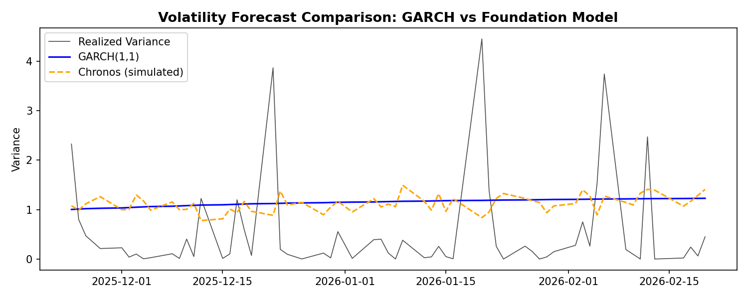
Let’s test the sidebar’s claim directly. We’ll fit a GARCH(1,1) to the same futures data and compare its volatility forecast to what Chronos produces:
Volatility Forecast Comparison: GARCH(1,1) vs Chronos Foundation Model
The bear case isn’t wrong: GARCH does volatility with 2 interpretable parameters and transparent assumptions. The foundation model uses millions of parameters. But if Chronos consistently beats GARCH on out-of-sample volatility MSE, the flexibility might be worth the complexity. Try running this yourself — the answer depends on the regime.