Internal Bar Strength (IBS) is an idea that has been around for some time. IBS is based on the position of the day’s close in relation to the day’s range: it takes a value of 0 if the closing price is the lowest price of the day, and 1 if the closing price is the highest price of the day.
More formally:
IBS = (Close – Low) / (High – Low)
The IBS effect may be related to intraday over-reaction to news or market movements, which are then ”corrected” the next day. It serves as a measure of the tendency of a price series to mean-revert over daily horizons. I use the term “daily” advisedly: so far as I am aware, there has been no research (including my own) demonstrating the existence of an IBS effect at time horizons shorter, or longer, than one day. Indeed, there has been very little in the way of academic research into the concept of any kind, which is strange considering how compelling are the results it is capable of producing. Practitioners have been happy enough with that state of affairs, content to deploy this neglected indicator in their trading strategies, where it has often proved to be extremely useful (we use IBS in one of our volatility strategies). Since 2013, however, the cat has been let out of the bag, thanks to an excellent research paper by Alexander Pagonidis, who writes an interesting quantitative finance blog.
The essence of the idea is that stocks that close in the lowest part of the daily range, with an IBS of below, say, 0.2, will tend to rally the next day, while stocks that close in the highest quintile will often decline in value in the following session. In his paper “The IBS Effect: Mean Reversion in Equity ETFs” (2013), Pagonidis researches the IBS effect in equity index ETFs in the US and several international markets. He confirms that low IBS values in these assets are associated with high returns in the following day session, while high IBS values are associated with low returns. Average returns when IBS is below 0.20 are .35% ,while average returns when IBS is above 0.80 are -0.13%. According to his research, this effect has been present in equity ETFs since the early 90s and has been highly consistent through time.

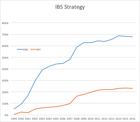
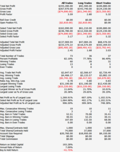
IBS Strategy Performance
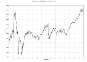
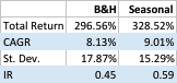
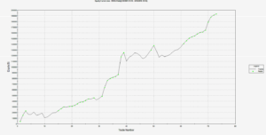
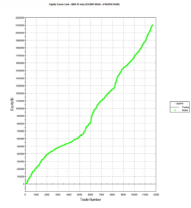
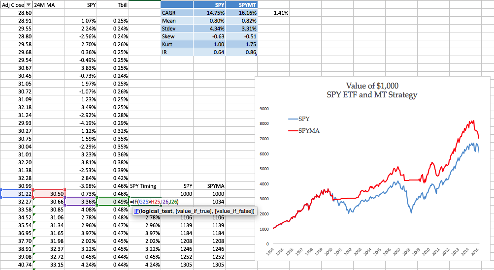
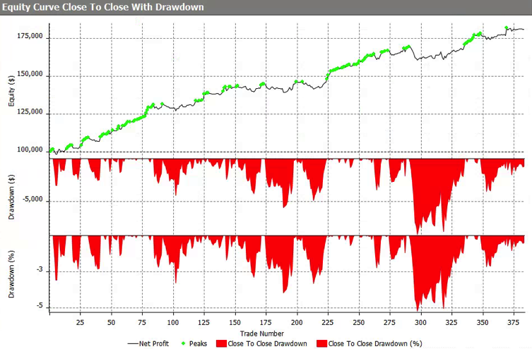
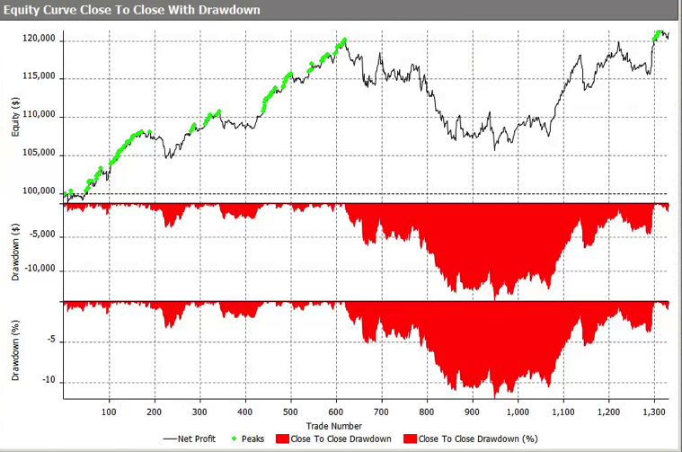
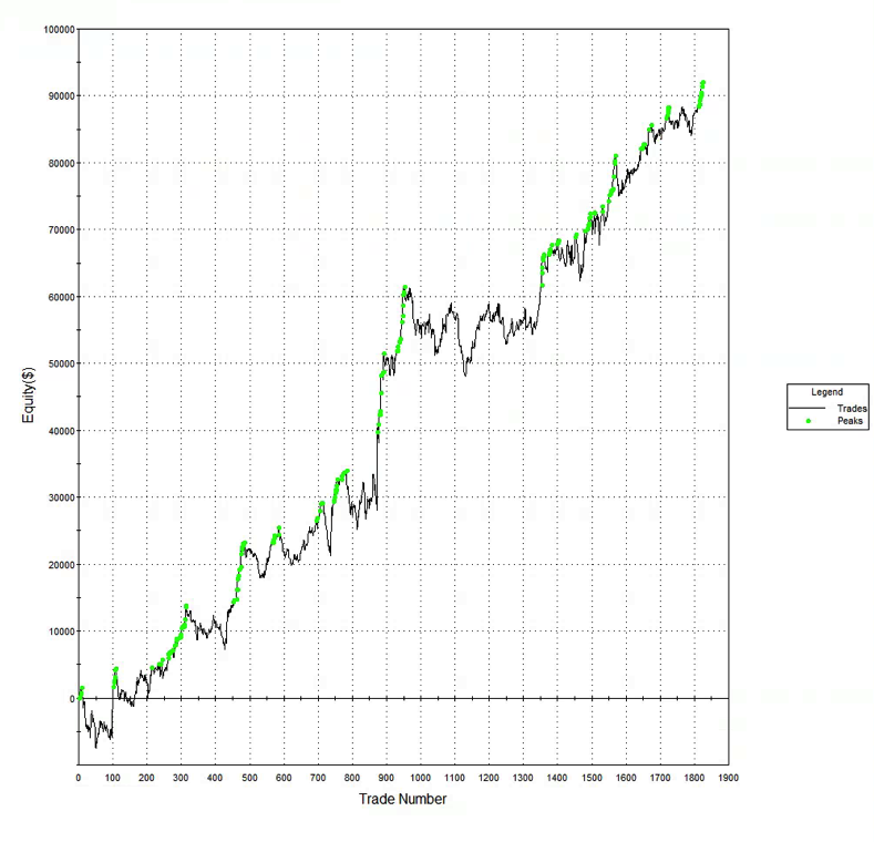
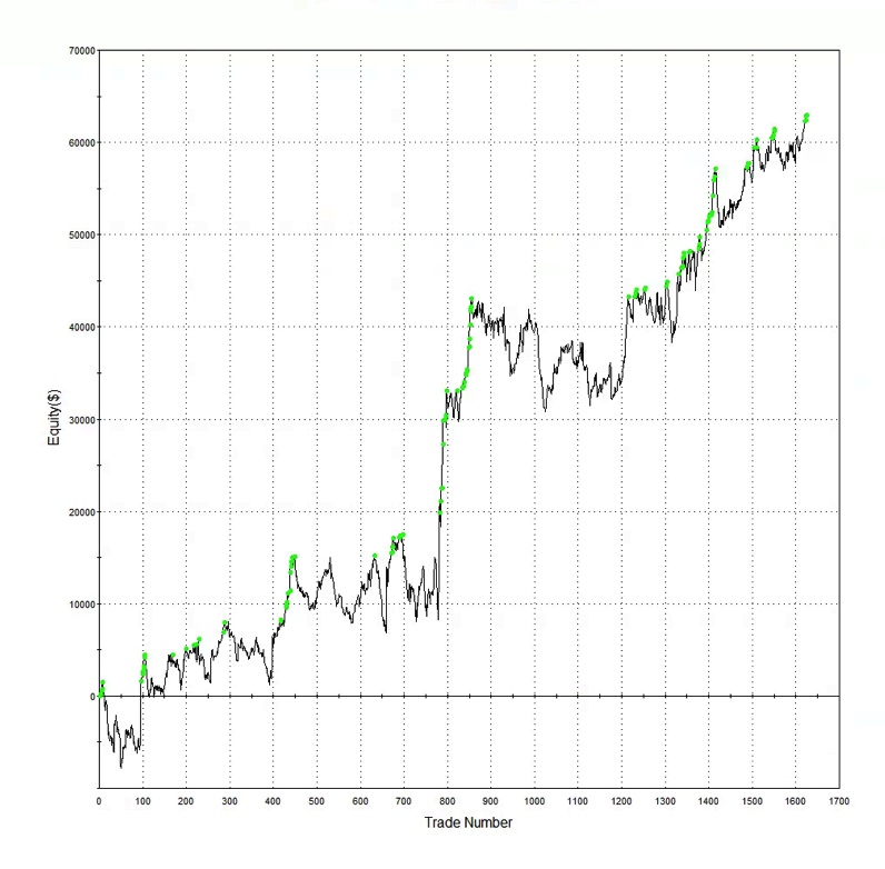
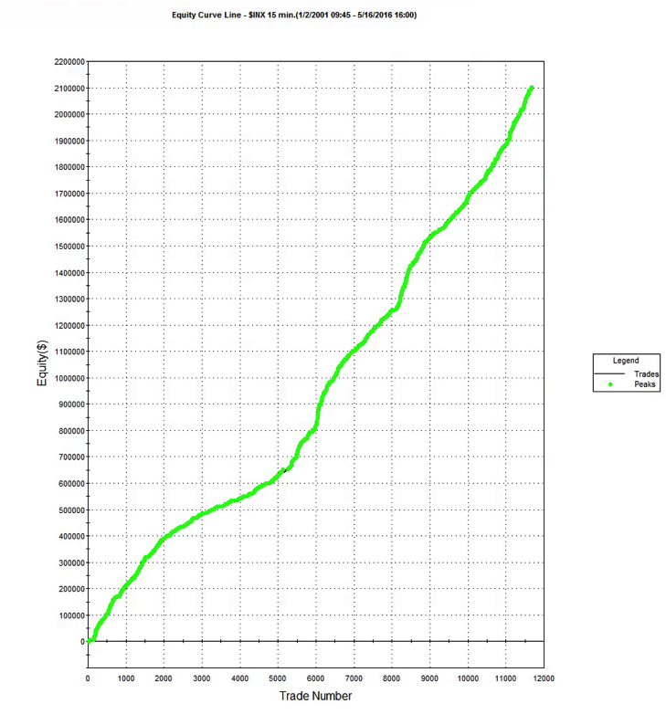
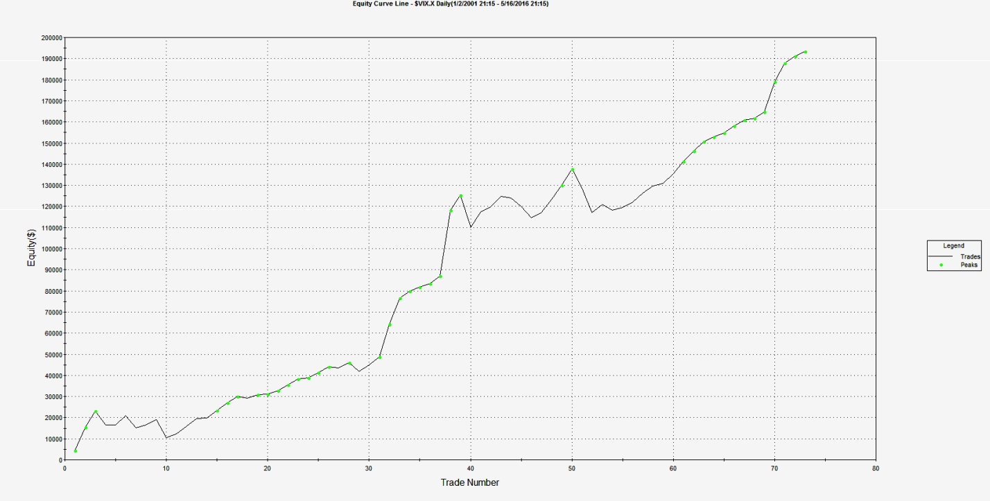
To give the reader some idea of the potential of the IBS effect, I have reproduced below equity curves for the IBS strategy for the SPDR S&P 500 ETF Trust (SPY) and iShares MSCI Singapore ETF (EWS) index ETFs over the period from 1999 to 2016. The strategy buys at the close when IBS is below 0.2, and sells at the close when IBS exceeds 0.8, liquidating the position at the following market close. Strategy CAGR over the period has been of the order of 13% for SPY and as high as 40% for EWS, ignoring transaction costs.
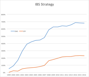
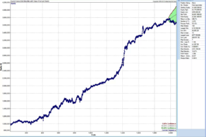
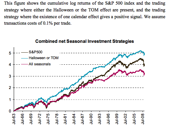
Note that in both cases strategy returns for SPY and EWS have diminished in recent years, turning negative in 2015 and 2016 YTD and this is true for ETFs in general. It remains to be seen whether this deterioration in strategy performance is temporary or permanent. There are some indications that the latter holds true, but the evidence is not quite definitive. For example, the chart below shows daily equity curve for the SPY IBS strategy, with 95% confidence intervals for the latest 100 trades (up to the end of May 2016), constructed using Monte-Carlo bootstrap. The equity curve appears to have penetrated the lower bound, indicating a statistically significant deterioration in the performance of the IBS strategy for SPY over the last year or so (EWS is similar). That said, the equity curve does fall inside the boundaries of the 99% confidence interval, so those looking for greater certainty about the possible breakdown of the effect will need to wait a little longer for confirmation.
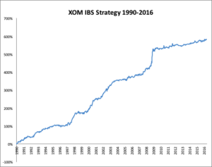
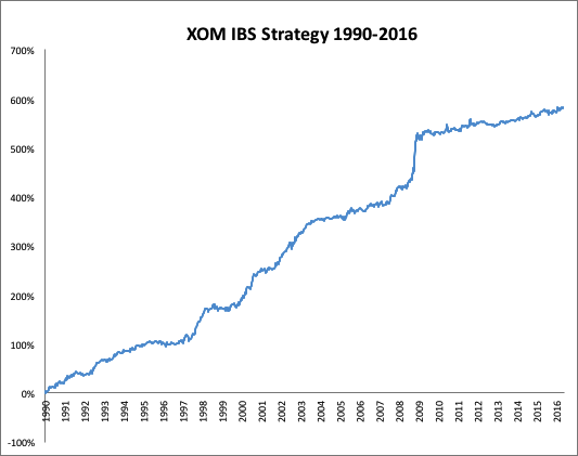
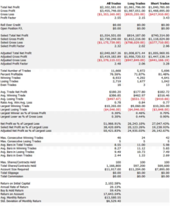
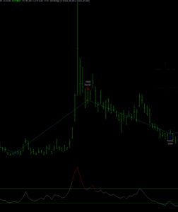
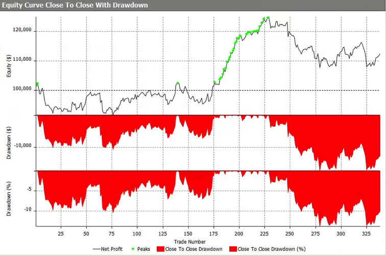
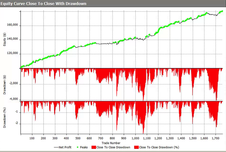
Whatever the outcome may be for SPY and other ETFs going forward, it is certainly true that IBS effects persist strongly for some individual equities, Exxon-Mobil Corp. (XOM) being a case in point (see below). It’s worth taking note of the exceptional performance of the XOM IBS strategy during the latter quarter of 2008. I will have much more to say on the application of the IBS indicator for individual equities in a future blog post.
The Role of Range, Volume, Bull/Bear Markets, Volatility and Seasonality
Pagonidis goes on to detail several further important findings in relation to IBS. It is clear from his research that high volatility is related to increased predictability of returns and a more powerful IBS effect, in particular the high IBS-negative return aspect. As might be expected, the effect is also larger after days with high range, both for high and low IBS extremes.
Volume turns out to be especially important for U.S. index ETFs: in fact, the IBS effect only appears to work on high-volume days.
Pagonidis also separates the data into bull and bear market environments, based on whether 200-day returns are positive or not. The size of the effect is roughly similar in each environment (slightly larger in bear markets), but it is greater in the direction of the overall trend: high IBS readings are followed by larger negative returns during bear markets, and vice versa.
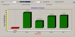
Day of Week Effect
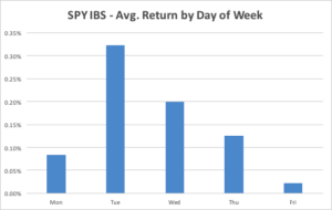
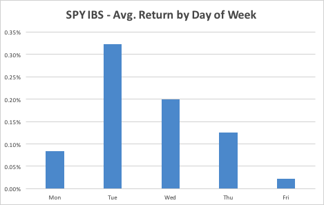
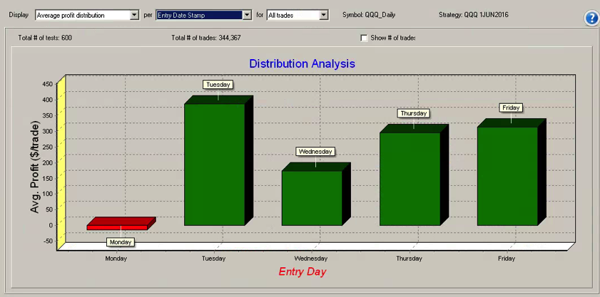
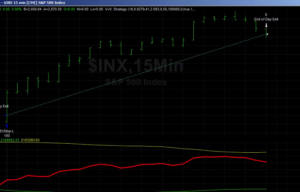
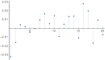
The IBS effect is also strongly seasonal, having the greatest impact on returns from Monday’s close to Tuesday’s close, as illustrated for the SPY ETF in the chart below. This accounts for the phenomenon known popularly as “Turnaround Tuesday”, i.e. the tendency for the market to recover strongly from losses on a Monday. The day-of-week effect is weakest for Fridays.
The mean of the returns distribution is not the only aspect that IBS can predict. Skewness also varies significantly between IBS buckets, with low IBS readings being followed by highly skewed returns, and vice versa. Close-to-close returns after a bottom-bucket IBS day have average skewness of 0.65 across Equity Index ETF products, while top-bucket IBS days are followed by returns with skewness of 0.03. This finding has very useful risk management applications for investors concerned with tail risk.
IBS as a Filter for a Swing Trading Strategy in QQQ
The returns to an IBS-only strategy are both statistically and economically significant. However, commissions will greatly decrease the returns and increase the maximum drawdowns, however, making such an approach challenging in the real world. One alternative is to combine the IBS effect with mean reversion on longer timescales and only take trades when they align.
Pagonidis offers a simple demonstration using the Cutler’s RSI indicator that shows how the IBS effect can be used to boost returns of a swing trading strategy while significantly decreasing the number of trades needed.
Cutler’s RSI at time t is calculated as follows:
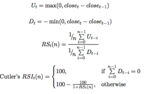
Pagonidis tests a simple, long-only strategy that trades the PowerShares QQQ Trust, Series 1 (QQQ) ETF using the Cutler’s RSI(3) indicator:
• Go long at the close if RSI(3) < 10
• Maintain the position while RSI(3) ≤ 40
filter these returns by adding an additional rule based on the value of IBS:
• Enter or maintain long position only if IBS ≤ 0.5
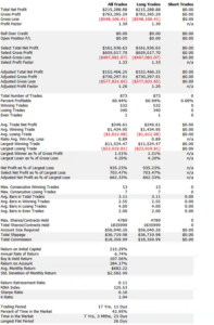
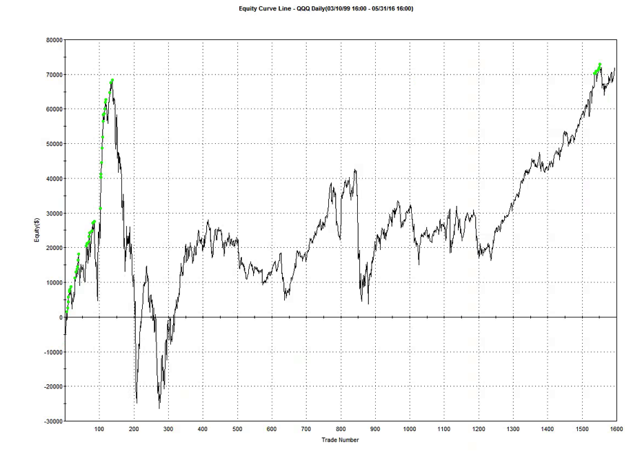
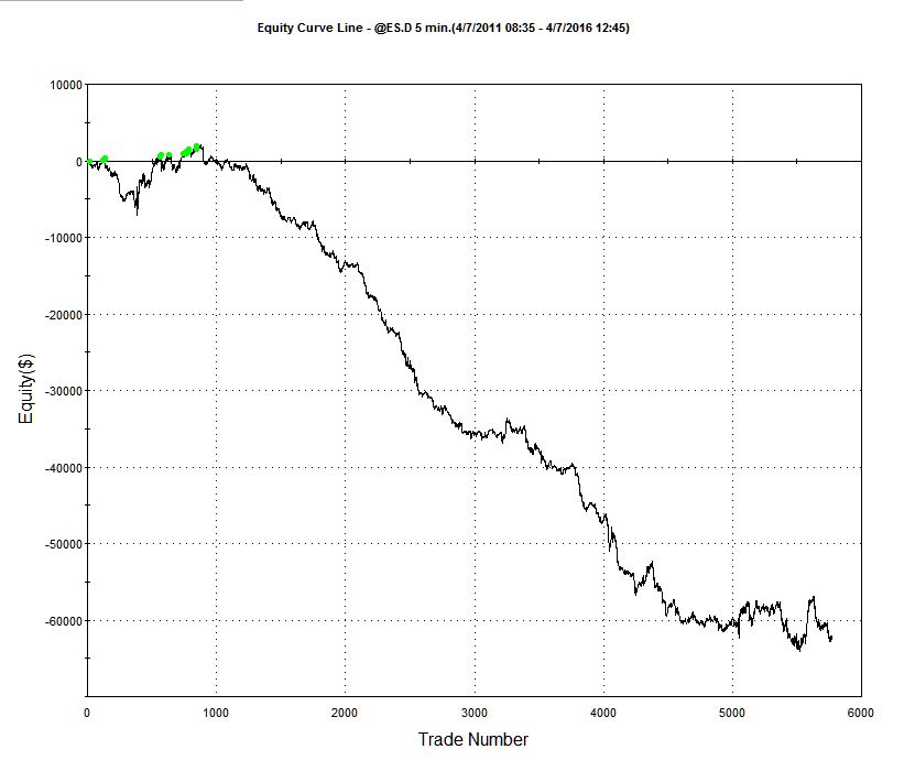
Pangonis claims that the strategy produces rather promising results that “easily beats commissions”; however, my own rendition of the strategy, assuming commissions of $0.005 per share and slippage of a further $0.02 per share produces results that are distinctly less encouraging:
Strategy Code
For those interested, the code is as follows:
Inputs:
RSILen(3),
RSI_Entry(10),
RSI_Exit(40),
IBS_Threshold(0.5),
Initial_Capital(100000);
Vars:
nShares(100),
RSIval(0),
IBS(0);
RSIval=RSI(C,RSILen);
IBS = (C-L)/(H-L);
nShares = Round(Initial_Capital / Close,0);
If Marketposition = 0 and RSIval > RSI_Entry and IBS < IBS_Threshold then begin
Buy nShares contracts next bar at market;
end;
If Marketposition > 0 and ((RSIval > RSI_Exit) or (IBS_Threshold > IBS_Threshold)) then begin
Sell next bar at market;
end;
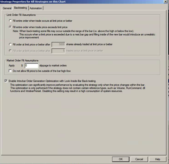
Strategy Optimization and Robustness Testing
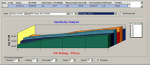
One can further improve performance by optimizing the trading system parameters, using Tradestation’s excellent Walk Forward Optimization (WFO) module. This allows us to examine the effect of re-calibrating the strategy parameters are regular intervals, testing the optimized model on out-of-sample data sets of various sizes. WFO can be used, not only optimize a strategy, but also to examine the sensitivity of its performance to changes in the levels of key parameters. For example, in the case of the QQQ swing trading strategy, we find that profitability increases monotonically with the length of the RSI indicator, and this effect is especially marked when an IBS threshold level of 0.2 is used:
Likewise we can test the consistency of the day-of-the-week effect over several OS data sets of varying size and these tests are consistent with the pattern seen earlier for the IBS indicator, confirming its role as a filter rule in enhancing system profitability:
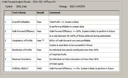
A model that is regularly re-calibrated using WFO is subjected to a series of tests designed to ensure its robustness and consistency in live trading. The tests include the following:
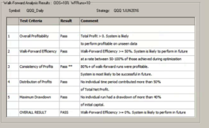
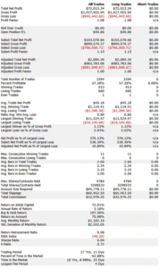
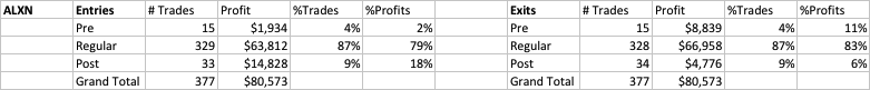
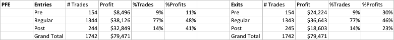
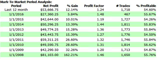
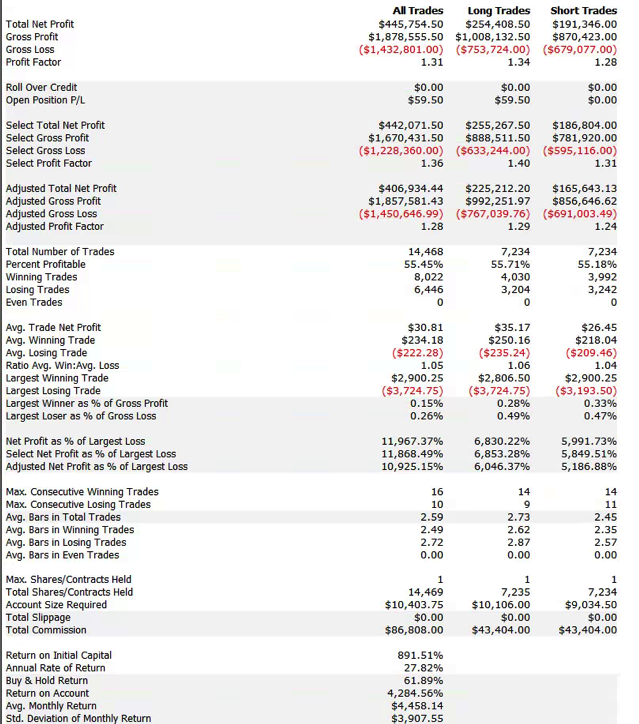
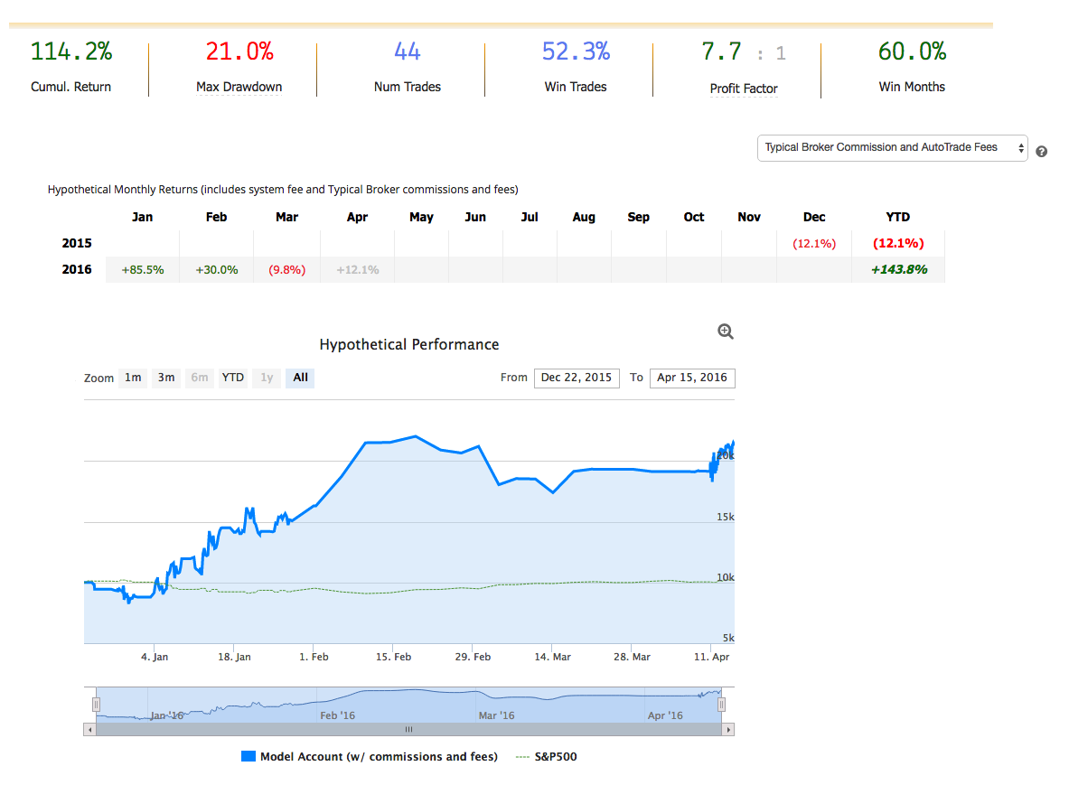
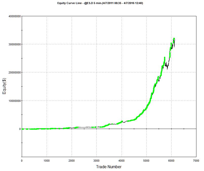
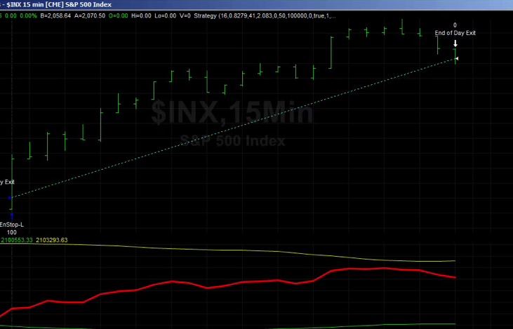
In order to achieve an overall pass rating, the system is required to pass all five tests of its out-of-sample performance, from which Tradestation deems it likely that the system will continue to perform well in live trading. The results from this procedure appear much more promising than the strategy in its original form, as can be seen from the performance table and equity curve chart shown below.
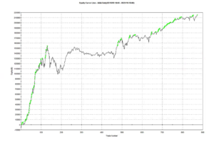
However, these results include both in-sample and out-of-sample periods. An examination of the results from the WFO indicate that the overall efficiency of the strategy is around 55%, meaning that the P&L produced by the system in out-of-sample periods amounts to a little over one half of the rate of profit produced during in-sample periods. Going forward, therefore, we might expect the performance of the system in live trading to be only around half as good as shown here. While this is still superior to the original system, it may not be considered good enough. Nonetheless, for the purpose of illustrating the benefits of the IBS indicator as a trade filter, it makes the point.
Another interesting example of an IBS-based trading strategy in the QQQ and SPY ETFs can be found in the following blog post.
Conclusion
Internal Bar Strength is a powerful mean-reversion indicator for equity products traded at daily frequencies, with a consistent effect that has continued from the 1990s through to the current decade. IBS can be used on its own in mean-reversion strategies that have worked well for both US equities and US and International equity index ETFs, or used as a trade filter when combined with other alpha signals.
While there is evidence of a weakening of the IBS effect since around 2013 this is not yet confirmed statistically (at the 99% confidence level) and may simply be the result of normal statistical variation in its efficacy.


