QUANTITATIVE RESEARCH AND TRADING

April 23, 2019

Trading the Presidential Election

There is a great deal of market lore related to the US presidential elections. It is generally held that elections are good for the market, regardless of whether the incoming president is Democrat or Republican. To examine this thesis, I gathered data on presidential elections since 1950, considering only the first term of each newly elected president. My reason for considering first terms only was twofold: firstly, it might be expected that a new president is likely to exert a greater influence during his initial term in office and secondly, the 2016 contest will likewise see the appointment of a new president (rather than the re-election of a current one).

Market Performance Post Presidential Elections

The table below shows the 11 presidential races considered, with sparklines summarizing the cumulative return in the S&P 500 Index in the 12 month period following the start of the presidential term of office. The majority are indeed upward sloping, as is the overall average.

A more detailed picture emerges from the following chart. It transpires that the generally positive “presidential effect” is due overwhelmingly to the stellar performance of the market during the first year of the Gerald Ford and Barack Obama presidencies. In both cases presidential elections coincided with the market nadir following, respectively, the 1973 oil crisis and 2008 financial crisis, after which the economy staged a strong recovery.

Democrat vs. Republican Presidencies

There is a marked difference in the average market performance during the first year of a Democratic presidency vs. a Republican presidency. Doubtless, plausible explanations for this disparity are forthcoming from both political factions. On the Republican side, it could be argued that Democratic presidents have benefitted from the benign policies of their (often) Republican predecessors, while incoming Republican presidents have had to clean up the mess left to them by their Democratic predecessors. Democrats would no doubt argue that the market, taking its customary forward view, tends to react favorably to the prospect of a more enlightened, liberal approach to the presidency (aka more government spending).

Market Performance Around the Start of Presidential Terms

I shall leave such political speculations to those interested in pursuing them and instead focus on matters of a more apolitical nature. Specifically, we will look at the average market returns during the twelve months leading up to the start of a new presidential term, compared to the average returns in the twelve months after the start of the term. The results are as follows:

The twelve months leading up to the start of the presidential term are labelled -12, -11, …, -1, while the following twelve months are labelled 1, 2, … , 12. The start of the term is designated as month zero, while months that fall outside the 24 month period around the start of a presidential term are labelled as month 13.

The key finding stands out clearly from the chart: namely, that market returns during the start month of a new presidential term are distinctly negative, averaging -3.3% , while returns in the first month after the start of the term are distinctly positive, averaging 2.81%.

Assuming that market returns are approximately Normally distributed, a standard t-test rejects the null hypothesis of no difference in the means of the month 0 and month 1 returns, at the 2% confidence level. In other words, the “presidential effect” is both large and statistically significant.

Conclusion: Trading the Election

Given the array of candidates before the electorate this election season, I am strongly inclined to take the trade. The market will certainly “feel the Bern” in the unlikely event that Bernie Sanders is elected president. I can even make an argument for a month 1 recovery, when the market realizes that there are limits to how much economic damage even a Socialist president can do, given constitutional checks and balances, “pen and phone” not withstanding.

Again, an incoming president Trump is likely to be greeted by a sharp market sell-off, based on jittery speculation about the Donald’s proclivity to start a trade war with China, or Mexico, or a ground war with Russia, Iran, or anyone else. Likewise, however, the market will fairly quickly come around to the realization that electioneering rhetoric is unlikely to provide much guidance as to what a president Trump is likely to do in practice.

A Hillary Clinton presidency is likely to be seen, ex-ante, as the most benign for the market, especially given the level of (financial) support she has received from Wall Street. However, there’s a glitch: Bernie is proving much tougher to shake off than she could ever have anticipated. In order to win over his supporters, she is going to have to move out of the center ground, towards the left. Who knows what hostages to fortune a desperate Clinton is likely to have to offer the election gods in her bid to secure the White House?

In terms of the mechanics, while you could take the trade in ETF’s or futures, this is one of those situations ideally suited to options and I am inclined to suggest combining a front-month put spread with a back-month call spread.

April 16, 2019

Yes, You Can Time the Market. How it Works, And Why

One of the most commonly cited maxims is that market timing is impossible. In fact, empirical evidence makes a compelling case that market timing is feasible and can yield substantial economic benefits. What’s more, we even understand why it works. For the typical portfolio investor, applying simple techniques to adjust their market exposure can prevent substantial losses during market downturns.

The Background From Empirical and Theoretical Research

For the last fifty years, since the work of Paul Samuelson, the prevailing view amongst economists has been that markets are (mostly) efficient and follow a random walk. Empirical evidence to the contrary was mostly regarded as anomalous and/or unimportant economically. Over time, however, evidence has accumulated that market effects may persist that are exploitable. The famous 1992 paper published by Fama and French, for example, identified important economic effects in stock returns due to size and value factors, while Cahart (1997) demonstrated the important incremental effect of momentum. The combined four-factor Cahart model explains around 50% of the variation in stock returns, but leaves a large proportion that cannot be accounted for.

Other empirical studies have provided evidence that stock returns are predictable at various frequencies. Important examples include work by Brock, Lakonishok and LeBaron (1992), Pesaran and Timmermann (1995) and Lo, Mamaysky and Wang (2000), who provide further evidence using a range of technical indicators with wide popularity among traders showing that this adds value even at the individual stock level over and above the performance of a stock index. The research in these and other papers tends to be exceptional in term of both quality and comprehensiveness, as one might expect from academics risking their reputations in taking on established theory. The appendix of test results to the Pesaran and Timmermann study, for example, is so lengthy that is available only in CD-ROM format.

A more recent example is the work of Paskalis Glabadanidis, in a 2012 paper entitled Market Timing with Moving Averages. Glabadanidis examines a simple moving average strategy that, he finds, produces economically and statistically significant alphas of 10% to 15% per year, after transaction costs, and which are largely insensitive to the four Cahart factors.

Glabadanidis reports evidence regarding the profitability of the MA strategy in seven international stock markets. The performance of the MA strategies also holds for more than 18,000 individual stocks. He finds that:

“The substantial market timing ability of the MA strategy appears to be the main driver of the abnormal returns.”

An Illustration of a Simple Marketing Timing Strategy in SPY

It is impossible to do justice to Glabadanidis’s research in a brief article and the interested reader is recommended to review the paper in full. However, we can illustrate the essence of the idea using the SPY ETF as an example.

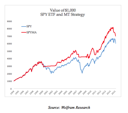
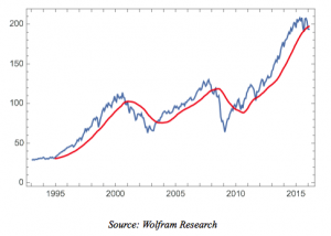
A 24-period moving average of the monthly price series over the period from 1993 to 2016 is plotted in red in the chart below.

The moving average indicator is used to time the market using the following simple rule:

if P_t >= MA_t invest in SPY in month t+1

if P_t < MA_t invest in T-bills in month t+1

In other words, we invest or remain invested in SPY when the monthly closing price of the ETF lies at or above the 24-month moving average, otherwise we switch our investment to T-Bills.

The process of switching our investment will naturally incur transaction costs and these are included in the net monthly returns.

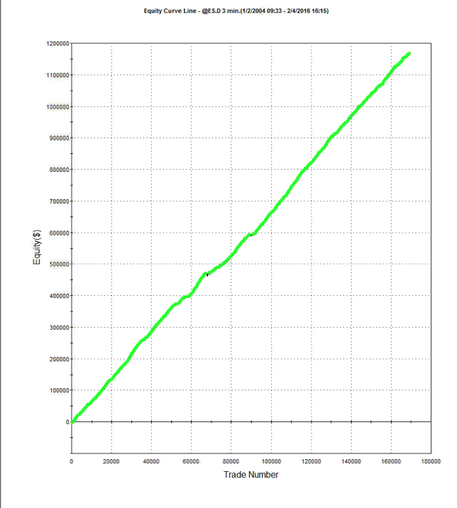
The outcome of the strategy in terms of compound growth is compared to the original long-only SPY investment in the following chart.

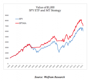
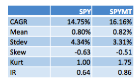
The marketing timing strategy outperforms the long-only ETF, with a CAGR of 16.16% vs. 14.75% (net of transaction costs), largely due to its avoidance of the major market sell-offs in 2000-2003 and 2008-2009.

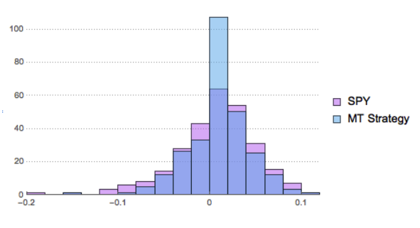
But the improvement isn’t limited to a 141bp improvement in annual compound returns. The chart below compares the distributions of monthly returns in the SPY ETF and market timing strategy.

It is clear that, in addition to a higher average monthly return, the market timing strategy has lower dispersion in the distribution in returns. This leads to a significantly higher information ratio for the strategy compared to the long-only ETF. Nor is that all: the market timing strategy has both higher skewness and kurtosis, both desirable features.

These results are entirely consistent with Glabadanidis’s research. He finds that the performance of the market timing strategy is robust to different lags of the moving average and in subperiods, while investor sentiment, liquidity risks, business cycles, up and down markets, and the default spread cannot fully account for its performance. The strategy works just as well with randomly generated returns and bootstrapped returns as it does for the more than 18,000 stocks in the study.

A follow-up study by the author applying the same methodology to a universe of 20 REIT indices and 274 individual REITs reaches largely similar conclusions.

Why Marketing Timing Works

For many investors, empirical evidence – compelling though it may be – is not enough to make market timing a credible strategy, absent some kind of “fundamental” explanation of why it works. Unusually, in the case of the simple moving average strategy, such explanation is possible.

It was Cox, Ross and Rubinstein who in 1979 developed the binomial model as a numerical method for pricing options. The methodology relies on the concept of option replication, in which one constructs a portfolio comprising holdings of the underlying stock and bonds to produce the same cash flows as the option at every point in time (the proportion of stock to hold is given by the option delta). Since the replicating portfolio produces the same cash flows as the option, it must have the same value and since once knows the price of the stock and bond at each point in time one can therefore price the option. For those interested in the detail, Wikipedia gives a detailed explanation of the technique.

We can apply the concept of option replication to construct something very close the MA market timing strategy, as follows. Consider what happens when the ETF falls below the moving average level. In that case we convert the ETF portfolio to cash and use the proceeds to acquire T-Bills. An equivalent outcome would be achieved by continuing to hold our long ETF position and acquiring a put option to hedge it. The combination of a long ETF position, and a 1-month put option with delta of -1, would provide the same riskless payoff as the market timing strategy, i.e. the return on 30-day T-Bills. An option in which the strike price is based on the average price of the underlying is known as an Arithmetic Asian option. Hence when we apply the MA timing strategy we are effectively constructing a dynamic portfolio that replicates the payoff of an Arithmetic Asian protective put option struck as (just above) the moving average level.

Market Timing Alpha and The Cost of Hedging

None of this explanation is particularly contentious – the theory behind option replication through dynamic hedging is well understood – and it provides a largely complete understanding of the way the MA market timing strategy works, one that should satisfy those who are otherwise unpersuaded by arguments purely from empirical research.

There is one aspect of the foregoing description that remains a puzzle, however. An option is a valuable financial instrument and the owner of a protective put of the kind described can expect to pay a price amounting to tens or perhaps hundreds of basis points. Of course, in the market timing strategy we are not purchasing a put option per se, but creating one synthetically through dynamic replication. The cost of creating this synthetic equivalent comprises the transaction costs incurred as we liquidate and re-assemble our portfolio from month to month, in the form of bid/ask spread and commissions. According to efficient market theory, one should be indifferent as to whether one purchases the option at a fair market price or constructs it synthetically through replication – the cost should be equivalent in either case. And yet in empirical tests the cost of the synthetic protective put falls far short of what one would expect to pay for an equivalent option instrument. This is, in fact, the source of the alpha in the market timing strategy.

According to efficient market theory one might expect to pay something of the order of 140 basis points a year in transaction costs – the difference between the CAGR of the market timing strategy and the SPY ETF – in order to construct the protective put. Yet, we find that no such costs are incurred.

Now, it might be argued that there is a hidden cost not revealed in our simple study of a market timing strategy applied to a single underlying ETF, which is the potential costs that could be incurred if the ETF should repeatedly cross and re-cross the level of the moving average, month after month. In those circumstances the transaction costs would be much higher than indicated here. The fact that, in a single example, such costs do not arise does not detract in any way from the potential for such a scenario to play out. Therefore, the argument goes, the actual costs from the strategy are likely to prove much higher over time, or when implemented for a large number of stocks.

All well and good, but this is precisely the scenario that Glabadanidis’s research addresses, by examining the outcomes, not only for tens of thousands of stocks, but also using a large number of scenarios generated from random and/or bootstrapped returns. If the explanation offered did indeed account for the hidden costs of hedging, it would have been evident in the research findings.

Instead, Glabadanidis concludes:

“This switching strategy does not involve any heavy trading when implemented with break-even transaction costs, suggesting that it will be actionable even for small investors.”

Implications For Current Market Conditions

As at the time of writing, in mid-February 2016, the price of the SPY ETF remains just above the 24-month moving average level. Consequently the market timing strategy implies one should continue to hold the market portfolio for the time being, although that could change very shortly, given recent market action.

Conclusion

The empirical evidence that market timing strategies produce significant alphas is difficult to challenge. Furthermore, we have reached an understanding of why they work, from an application of widely accepted option replication theory. It appears that using a simple moving average to time market entries and exits is approximately equivalent to hedging a portfolio with a protective Arithmetic Asian put option.

What remains to be answered is why the cost of constructing put protection synthetically is so low. At the current time, research indicates that market timing strategies consequently are able to generate alphas of 10% to 15% per annum.

References

Brock, W., Lakonishok, J., LeBaron, B., 1992, “Simple Technical Trading Rules and the Stochastic Properties of Stock Returns,” Journal of Finance 47, pp. 1731-1764.
Carhart, M. M., 1997, “On Persistence in Mutual Fund Performance,” Journal of Finance 52, pp. 57–82.
Fama, E. F., French, K. R., 1992, “The Cross-Section of Expected Stock Returns,” Journal of Finance 47(2), 427–465
Glabadanidis, P., 2012, “Market Timing with Moving Averages”, 25th Australasian Finance and Banking Conference.
Glabadanidis, P., 2012, “The Market Timing Power of Moving Averages: Evidence from US REITs and REIT Indexes”, University of Adelaide Business School.
Lo, A., Mamaysky, H., Wang, J., 2000, “Foundations of Technical Analysis: Computational Algorithms, Statistical Inference, and Empirical Implementation,” Journal of Finance 55, 1705–1765.
Pesaran, M.H., Timmermann, A.G., 1995, “Predictability of Stock Returns: Robustness and Economic Significance”, Journal of Finance, Vol. 50 No. 4

April 9, 2019

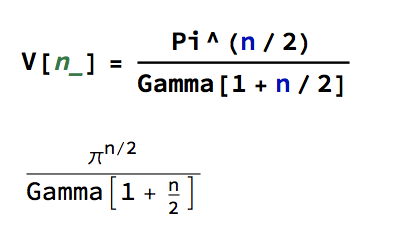
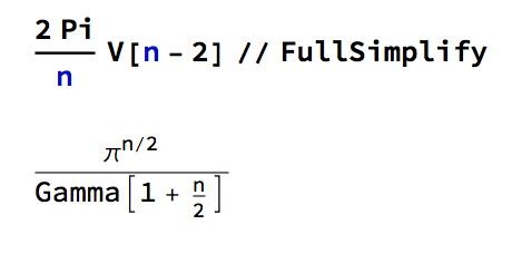
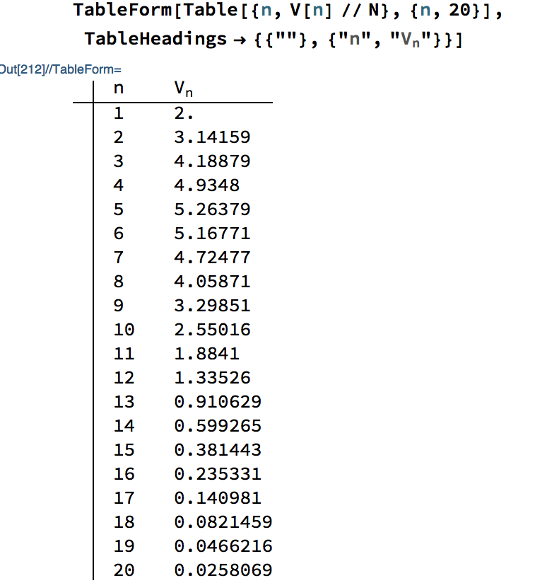
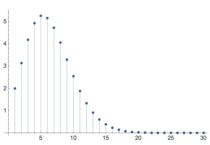
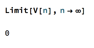
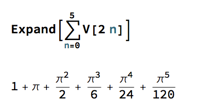
Profit Margins – Are they Predicting a Crash?

Jeremy Grantham: A Bullish Bear

Is Jeremy Grantham, co-founder and CIO of GMO, bullish or bearish these days? According to Myles Udland at Business Insider, he’s both. He quotes Grantham:

“I think the global economy and the U.S. in particular will do better than the bears believe it will because they appear to underestimate the slow-burning but huge positive of much-reduced resource prices in the U.S. and the availability of capacity both in labor and machinery.”

Udland continues:

“On top of all this is the decline in profit margins, which Grantham has called the “most mean-reverting series in finance,” implying that the long period of elevated margins we’ve seen from American corporations is most certainly going to come an end. And soon. “

Corporate Profit Margins as a Leading Indicator

The claim is an interesting one. It certainly looks as if corporate profit margins are mean-reverting and, possibly, predictive of recessionary periods. And there is an economic argument why this should be so, articulated by Grantham as quoted in an earlier Business Insider article by Sam Ro:

“Profit margins are probably the most mean-reverting series in finance, and if profit margins do not mean-revert, then something has gone badly wrong with capitalism.

If high profits do not attract competition, there is something wrong with the system and it is not functioning properly.”

Thomson Research / Barclays Research’s take on the same theme echoes Grantham:

“The link between profit margins and recessions is strong,” Barclays’ Jonathan Glionna writes in a new note to clients. “We analyze the link between profit margins and recessions for the last seven business cycles, dating back to 1973. The results are not encouraging for the economy or the market. In every period except one, a 0.6% decline in margins in 12 months coincided with a recession.”

Buffett Weighs in

Even Warren Buffett gets in on the act (from 1999):

“In my opinion, you have to be wildly optimistic to believe that corporate profits as a percent of GDP can, for any sustained period, hold much above 6%.”

With the Illuminati chorusing as one on the perils of elevated rates of corporate profits, one would be foolish to take a contrarian view, perhaps. And yet, that claim of Grantham’s (“probably the most mean-reverting series in finance”) poses a challenge worthy of some analysis. Let’s take a look.

The Predictive Value of Corporate Profit Margins

First, let’s reproduce the St Louis Fed chart:

A plot of the series autocorrelations strongly suggests that the series is not at all mean-reverting, but non-stationary, integrated order 1:

Next, we conduct an exhaustive evaluation of a wide range of time series models, including seasonal and non-seasonal ARIMA and GARCH:

The best fitting model (using the AIC criterion) is a simple ARMA(0,1,0) model, integrated order 1, as anticipated. The series is apparently difference-stationary, with no mean-reversion characteristics at all. Diagnostic tests indicate no significant patterning in the model residuals:

LjungPlot — Ljung-Box Test Probabilities

Using the model to forecast a range of possible values of the Corporate Profit to GDP ratio over the next 8 quarters suggests a very wide range, from as low as 6% to as high as 13%!

CONCLUSION

The opinion of investment celebrities like Grantham and Buffett to the contrary, there really isn’t any evidence in the data to support the suggestion that corporate profit margins are mean reverting, even though common-sense economics suggests they should be.

The best-available econometric model produces a very wide range of forecasts of corporate profit rates over the next two years, some even higher than they are today.

If a recession is just around the corner, corporate profit margins aren’t going to call it for us.

April 2, 2019

Alpha Extraction and Trading Under Different Market Regimes

Market Noise and Alpha Signals

One of the perennial problems in designing trading systems is noise in the data, which can often drown out an alpha signal. This is turn creates difficulties for a trading system that relies on reading the signal, resulting in greater uncertainty about the trading outcome (i.e. greater volatility in system performance). According to academic research, a great deal of market noise is caused by trading itself. There is apparently not much that can be done about that problem: sure, you can trade after hours or overnight, but the benefit of lower signal contamination from noise traders is offset by the disadvantage of poor liquidity. Hence the thrust of most of the analysis in this area lies in the direction of trying to amplify the signal, often using techniques borrowed from signal processing and related engineering disciplines.

There is, however, one trick that I wanted to share with readers that is worth considering. It allows you to trade during normal market hours, when liquidity is greatest, but at the same time limits the impact of market noise.

Quantifying Market Noise

How do you measure market noise? One simple approach is to start by measuring market volatility, making the not-unreasonable assumption that higher levels of volatility are associated with greater amounts of random movement (i.e noise). Conversely, when markets are relatively calm, a greater proportion of the variation is caused by alpha factors. During the latter periods, there is a greater information content in market data – the signal:noise ratio is larger and hence the alpha signal can be quantified and captured more accurately.

For a market like the E-Mini futures, the variation in daily volatility is considerable, as illustrated in the chart below. The median daily volatility is 1.2%, while the maximum value (in 2008) was 14.7%!

The extremely long tail of the distribution stands out clearly in the following histogram plot.

Obviously there are times when the noise in the process is going to drown out almost any alpha signal. What if we could avoid such periods?

Noise Reduction and Model Fitting

Let’s divide our data into two subsets of equal size, comprising days on which volatility was lower, or higher, than the median value. Then let’s go ahead and use our alpha signal(s) to fit a trading model, using only data drawn from the lower volatility segment.

This is actually a little tricky to achieve in practice: most software packages for time series analysis or charting are geared towards data occurring at equally spaced points in time. One useful trick here is to replace the actual date and time values of the observations with sequential date and time values, in order to fool the software into accepting the data, since there are no longer any gaps in the timestamps. Of course, the dates on our time series plot or chart will be incorrect. But that doesn’t matter: as long as we know what the correct timestamps are.

An example of such a system is illustrated below. The model was fitted to 3-Min bar data in EMini futures, but only on days with market volatility below the median value, in the period from 2004 to 2015. The strategy equity curve is exceptionally smooth, as might be expected, and the performance characteristics of the strategy are highly attractive, with a 27% annual rate of return, profit factor of 1.58 and Sharpe Ratio approaching double-digits.

Dealing with the Noisy Trading Days

Let’s say you have developed a trading system that works well on quiet days. What next? There are a couple of ways to go:

(i) Deploy the model only on quiet trading days; stay out of the market on volatile days; or

(ii) Develop a separate trading system to handle volatile market conditions.

Which approach is better? It is likely that the system you develop for trading quiet days will outperform any system you manage to develop for volatile market conditions. So, arguably, you should simply trade your best model when volatility is muted and avoid trading at other times. Any other solution may reduce the overall risk-adjusted return. But that isn’t guaranteed to be the case – and, in fact, I will give an example of systems that, when combined, will in practice yield a higher information ratio than any of the component systems.

Deploying the Trading Systems

The astute reader is likely to have noticed that I have “cheated” by using forward information in the model development process. In building a trading system based only on data drawn from low-volatility days, I have assumed that I can somehow know in advance whether the market is going to be volatile or not, on any given day. Of course, I don’t know for sure whether the upcoming session is going to be volatile and hence whether to deploy my trading system, or stand aside. So is this just a purely theoretical exercise? No, it’s not, for the following reasons.

The first reason is that, unlike the underlying asset market, the market volatility process is, by comparison, highly predictable. This is due to a phenomenon known as “long memory”, i.e. very slow decay in the serial autocorrelations of the volatility process. What that means is that the history of the volatility process contains useful information about its likely future behavior. [There are several posts on this topic in this blog – just search for “long memory”]. So, in principle, one can develop an effective system to forecast market volatility in advance and hence make an informed decision about whether or not to deploy a specific model.

But let’s say you are unpersuaded by this argument and take the view that market volatility is intrinsically unpredictable. Does that make this approach impractical? Not at all. You have a couple of options:

You can test the model built for quiet days on all the market data, including volatile days. It may perform acceptably well across both market regimes.

For example, here are the results of a backtest of the model described above on all the market data, including volatile and quiet periods, from 2004-2015. While the performance characteristics are not quite as good, overall the strategy remains very attractive.

Another approach is to develop a second model for volatile days and deploy both low- and high-volatility regime models simultaneously. The trading systems will interact (if you allow them to) in a highly nonlinear and unpredictable way. It might turn out badly – but on the other hand, it might not! Here, for instance, is the result of combining low- and high-volatility models simultaneously for the Emini futures and running them in parallel. The result is an improvement (relative to the low volatility model alone), not only in the annual rate of return (21% vs 17.8%), but also in the risk-adjusted performance, profit factor and average trade.

CONCLUSION

Separating the data into multiple subsets representing different market regimes allows the system developer to amplify the signal:noise ratio, increasing the effectiveness of his alpha factors. Potentially, this allows important features of the underlying market dynamics to be captured in the model more easily, which can lead to improved trading performance.

Models developed for different market regimes can be tested across all market conditions and deployed on an everyday basis if shown to be sufficiently robust. Alternatively, a meta-strategy can be developed to forecast the market regime and select the appropriate trading system accordingly.

Finally, it is possible to achieve acceptable, or even very good results, by deploying several different models simultaneously and allowing them to interact, as the market moves from regime to regime.

March 26, 2019

How to Make Money in a Down Market

The popular VIX blog Vix and More evaluates the performance of the VIX ETFs (actually ETNs) and concludes that all of them lost money in 2015. Yes, both long volatility and short volatility products lost money!

Source: Vix and More

By contrast, our Volatility ETF strategy had an exceptional year in 2015, making money in every month but one:

How to Profit in a Down Market

How do you make money when every product you are trading loses money? Obviously you have to short one or more of them. But that can be a very dangerous thing to do, especially in a product like the VIX ETNs. Volatility itself is very volatile – it has an annual volatility (the volatility of volatility, or VVIX) that averages around 100% and which reached a record high of 212% in August 2015.

The CBOE VVIX Index

Selling products based on such a volatile instrument can be extremely hazardous – even in a downtrend: the counter-trends are often extremely violent, making a short position challenging to maintain.

Relative value trading is a more conservative approach to the problem. Here, rather than trading a single product you trade a pair, or basket of them. Your bet is that the ETFs (or stocks) you are long will outperform the ETFs you are short. Even if your favored ETFs declines, you can still make money if the ETFs you short declines even more.

This is the basis for the original concept of hedge funds, as envisaged by Alfred Jones in the 1940’s, and underpins the most popular hedge fund strategy, equity long-short. But what works successfully in equities can equally be applied to other markets, including volatility. In fact, I have argued elsewhere that the relative value (long/short) concept works even better in volatility markets, chiefly because the correlations between volatility processes tend to be higher than the correlations between the underlying asset processes (see The Case for Volatility as an Asset Class).

March 14, 2019

Protected: Systematic Fund

March 12, 2019

Overnight Trading in the E-Mini S&P 500 Futures

Jeff Swanson’s Trading System Success web site is often worth a visit for those looking for new trading ideas.

A recent post Seasonality S&P Market Session caught my eye, having investigated several ideas for overnight trading in the E-minis. Seasonal effects are of course widely recognized and traded in commodities markets, but they can also apply to financial products such as the E-mini. Jeff’s point about session times is well-made: it is often worthwhile to look at the behavior of an asset, not only in different time frames, but also during different periods of the trading day, day of the week, or month of the year.

Jeff breaks the E-mini trading session into several basic sub-sessions:

“Pre-Market” Between 530 and 830
“Open” Between 830 and 900
“Morning” Between 900 though 1130
“Lunch” Between 1130 and 1315
“Afternoon” Between 1315 and 1400
“Close” Between 1400 and 1515
“Post-Market” Between 1515 and 1800
“Night” Between 1800 and 530

In his analysis Jeff’s strategy is simply to buy at the open of the session and close that trade at the conclusion of the session. This mirrors the traditional seasonality study where a trade is opened at the beginning of the season and closed several months later when the season comes to an end.

Evaluating Overnight Session and Seasonal Effects

The analysis evaluates the performance of this basic strategy during the “bullish season”, from Nov-May, when the equity markets traditionally make the majority of their annual gains, compared to the outcome during the “bearish season” from Jun-Oct.

None of the outcomes of these tests is especially noteworthy, save one: the performance during the overnight session in the bullish season:

The tendency of the overnight session in the E-mini to produce clearer trends and trading signals has been well documented. Plausible explanations for this phenomenon are that:

(a) The returns process in the overnight session is less contaminated with noise, which primarily results from trading activity; and/or

(b) The relatively poor liquidity of the overnight session allows participants to push the market in one direction more easily.

Either way, there is no denying that this study and several other, similar studies appear to demonstrate interesting trading opportunities in the overnight market.

That is, until trading costs are considered. Results for the trading strategy from Nov 1997-Nov 2015 show a gain of $54,575, but an average trade of only just over $20:

Gross PL	# Trades	Av Trade
$54,575	2701	$20.21

Assuming that we enter and exit aggressively, buying at the market at the start of the session and selling MOC at the close, we will pay the bid-offer spread and commissions amounting to around $30, producing a net loss of $10 per trade.

The situation can be improved by omitting January from the “bullish season”, but the slightly higher average trade is still insufficient to overcome trading costs :

Gross PL	# Trades	Av Trade
$54,550	2327	$23.44

Designing a Seasonal Trading Strategy for the Overnight Session

At this point an academic research paper might conclude that the apparently anomalous trading profits are subsumed within the bid-offer spread. But for a trading system designer this is not the end of the story.

If the profits are insufficient to overcome trading frictions when we cross the spread on entry and exit, what about a trading strategy that permits market orders on only the exit leg of the trade, while using limit orders to enter? Total trading costs will be reduced to something closer to $17.50 per round turn, leaving a net profit of almost $6 per trade.

Of course, there is no guarantee that we will successfully enter every trade – our limit orders may not be filled at the bid price and, indeed, we are likely to suffer adverse selection – i.e. getting filled on every losing trading, while missing a proportion of the winning trades.

On the other hand, we are hardly obliged to hold a position for the entire overnight session. Nor are we obliged to exit every trade MOC – we might find opportunities to exit prior to the end of the session, using limit orders to achieve a profit target or cap a trading loss. In such a system, some proportion of the trades will use limit orders on both entry and exit, reducing trading costs for those trades to around $5 per round turn.

The key point is that we can use the seasonal effects detected in the overnight session as a starting point for the development for a more sophisticated trading system that uses a variety of entry and exit criteria, and order types.

The following shows the performance results for a trading system designed to trade 30-minute bars in the E-mini futures overnight session during the months of Nov to May.The strategy enters trades using limit prices and exits using a combination of profit targets, stop loss targets, and MOC orders.

Data from 1997 to 2010 were used to design the system, which was tested on out-of-sample data from 2011 to 2013. Unseen data from Jan 2014 to Nov 2015 were used to provide a further (double blind) evaluation period for the strategy.

	ALL TRADES	LONG	SHORT
Closed Trade Net Profit	$83,080	$61,493	$21,588
Gross Profit	$158,193	$132,573	$25,620
Gross Loss	-$75,113	-$71,080	-$4,033
Profit Factor	2.11	1.87	6.35
Ratio L/S Net Profit	2.85
Total Net Profit	$83,080	$61,493	$21,588
Trading Period	11/13/97 2:30:00 AM to 12/31/13 6:30:00 AM (16 years 48 days)
Number of Trading Days	2767
Starting Account Equity	$100,000
Highest Equity	$183,080
Lowest Equity	$97,550
Final Closed Trade Equity	$183,080
Return on Starting Equity	83.08%
Number of Closed Trades	849	789	60
Number of Winning Trades	564	528	36
Number of Losing Trades	285	261	24
Trades Not Taken	0	0	0
Percent Profitable	66.43%	66.92%	60.00%
Trades Per Year	52.63	48.91	3.72
Trades Per Month	4.39	4.08	0.31
Max Position Size	1	1	1
Average Trade (Expectation)	$97.86	$77.94	$359.79
Average Trade (%)	0.07%	0.06%	0.33%
Trade Standard Deviation	$641.97	$552.56	$1,330.60
Trade Standard Deviation (%)	0.48%	0.44%	1.20%
Average Bars in Trades	15.2	14.53	24.1
Average MAE	$190.34	$181.83	$302.29
Average MAE (%)	0.14%	0.15%	0.27%
Maximum MAE	$3,237	$2,850	$3,237
Maximum MAE (%)	2.77%	2.52%	3.10%
Win/Loss Ratio	1.06	0.92	4.24
Win/Loss Ratio (%)	2.10	1.83	7.04
Return/Drawdown Ratio	15.36	14.82	5.86
Sharpe Ratio	0.43	0.46	0.52
Sortino Ratio	1.61	1.69	6.40
MAR Ratio	0.71	0.73	0.33
Correlation Coefficient	0.95	0.96	0.719
Statistical Significance	100%	100%	97.78%
Average Risk	$1,099	$1,182	$0.00
Average Risk (%)	0.78%	0.95%	0.00%
Average R-Multiple (Expectancy)	0.0615	0.0662	0
R-Multiple Standard Deviation	0.4357	0.4357	0
Average Leverage	0.399	0.451	0.463
Maximum Leverage	0.685	0.694	0.714
Risk of Ruin	0.00%	0.00%	0.00%
Kelly f	34.89%	31.04%	50.56%
Average Annual Profit/Loss	$5,150	$3,811	$1,338
Ave Annual Compounded Return	3.82%	3.02%	1.22%
Average Monthly Profit/Loss	$429.17	$317.66	$111.52
Ave Monthly Compounded Return	0.31%	0.25%	0.10%
Average Weekly Profit/Loss	$98.70	$73.05	$25.65
Ave Weekly Compounded Return	0.07%	0.06%	0.02%
Average Daily Profit/Loss	$30.03	$22.22	$7.80
Ave Daily Compounded Return	0.02%	0.02%	0.01%
INTRA-BAR EQUITY DRAWDOWNS	ALL TRADES	LONG	SHORT
Number of Drawdowns	445	422	79
Average Drawdown	$282.88	$269.15	$441.23
Average Drawdown (%)	0.21%	0.20%	0.33%
Average Length of Drawdowns	10 days 19 hours	10 days 20 hours	66 days 1 hours
Average Trades in Drawdowns	3	3	1
Worst Case Drawdown	$6,502	$4,987	$4,350
Date at Trough	12/13/00 1:30	5/24/00 4:30	12/13/00 1:30

March 5, 2019

Improving A Hedge Fund Investment – Cantab Capital’s Quantitative Aristarchus Fund

In this post I am going to take a look at what an investor can do to improve a hedge fund investment through the use of dynamic capital allocation. For the purposes of illustration I am going to use Cantab Capital’s Aristarchus program – a quantitative fund which has grown to over $3.5Bn in assets under management since its opening with $30M in 2007 by co-founders Dr. Ewan Kirk and Erich Schlaikjer.

I chose this product because, firstly, it is one of the most successful quantitative funds in existence and, secondly, because as a CTA its performance record is publicly available.

Cantab’s Aristarchus Fund

Cantab’s stated investment philosophy is that algorithmic trading can help to overcome cognitive biases inherent in human-based trading decisions, by exploiting persistent statistical relationships between markets. Taking a multi-asset, multi-model approach, the majority of Cantab’s traded instruments are liquid futures and forwards, across currencies, fixed income, equity indices and commodities.

Let’s take a look at how that has worked out in practice:

Whatever the fund’s attractions may be, we can at least agree that alpha is not amongst them. A Sharpe ratio of < 0.5 (I calculate to be nearer 0.41) is hardly in Renaissance territory, so one imagines that the chief benefit of the product must lie in its liquidity and low market correlation. Uncorrelated it may be, but an investor in the fund must have extremely deep pockets – and a very strong stomach – to handle the 34% drawdown that the fund suffered in 2013.

Improving the Aristarchus Fund Performance

If we make the assumption that an investment in this product is warranted in the first place, what can be done to improve its performance characteristics? We’ll look at that question from two different perspectives – the investor’s and the manager’s.

Firstly, from the investor’s perspective, there are relatively few options available to enhance the fund’s contribution, other than through diversification. One other possibility available to the investor, however, is to develop a program for dynamic capital allocation. This requires the manager to be open to allowing significant changes in the amount of capital to be allocated from month to month, or quarter to quarter, but in a liquid product like Aristarchus some measure of flexibility ought to be feasible.

An analysis of the fund’s performance indicates the presence of a strong dependency in the returns process. This is not at all unusual. Often investment strategies have a tendency to mean-revert: a negative dependency in which periods of poor performance tend to be followed by positive performance, and vice versa. CTA strategies such as Aristarchus tend to be trend-following, and this can induce positive dependency in the strategy returns process, in which positive months tend to follow earlier positive months, while losing months tend to be followed by further losses. This is the pattern we find here.

Consequently, rather than maintaining a constant capital allocation, an investor would do better to allocate capital dynamically, increasing the amount of capital after a positive period, while decreasing the allocation after a period of losses. Let’s consider a variation of this allocation plan, in which the amount of allocated capital is increased by 70% when the last monthly equity value exceeds the quarterly moving average, while the allocation is reduced to zero when the last month’s equity falls below the average. A dynamic capital allocation plan as simple as this appears to produce a significant improvement in the overall performance of the investment:

The slight increase in annual volatility in the returns produced by the dynamic capital allocation model is more than offset by the 412bp improvement in the CAGR. Consequently, the Sharpe Ratio improves from o.41 to 0.60.

Nor is this by any means the entire story: the dynamic model produces lower average drawdowns (7.93% vs. 8.52%) and, more importantly, reduces the maximum drawdown over the life of the fund from a painful 34.87% to more palatable 23.92%.

The much-improved risk profile of the dynamic allocation scheme is reflected in the Return/Drawdown Ratio, which rises from 2.44 to 6.52.

Note, too, that the average level of capital allocated in the dynamic scheme is very slightly less than the original static allocation. In other words, the dynamic allocation technique results in a more efficient use of capital, while at the same time producing a higher rate of risk-adjusted return and enhancing the overall risk characteristics of the strategy.

Improving Fund Performance Using a Meta-Strategy

So much for the investor. What could the manager to do improve the strategy performance? Of course, there is nothing in principle to prevent the manager from also adopting a dynamic approach to capital allocation, although his investment mandate may require him to be fully invested at all times.

Assuming for the moment that this approach is not available to the manager, he can instead look into the possibilities for developing a meta-strategy. As I explained in my earlier post on the topic:

A meta-strategy is a trading system that trades trading systems. The idea is to develop a strategy that will make sensible decisions about when to trade a specific system, in a way that yields superior performance compared to simply following the underlying trading system.

It turns out to be quite straightforward to develop such a meta-strategy, using a combination of stop-loss limits and profit targets to decide when to turn the strategy on or off. In so doing, the manager is able to avoid some periods of negative performance, producing a significant uplift in the overall risk-adjusted return:

Conclusion

Meta-strategies and dynamic capital allocation schemes can enable the investor and the investment manager to improve the performance characteristics of their investment and investment strategy, by increasing returns, reducing volatility and the propensity of the strategy to produce substantial drawdowns.

We have demonstrated how these approaches can be applied successfully to Cantab’s Aristarchus quantitative fund, producing substantial gains in risk adjusted performance and reductions in the average and maximum drawdowns produced over the life of the fund.

February 21, 2019February 23, 2019

Pairs Trading – Part 2: Practical Considerations

Pairs Trading = Numbers Game

One of the first things you quickly come to understand in equity pairs trading is how important it is to spread your risk. The reason is obvious: stocks are subject to a multitude of risk factors – amongst them earning shocks and corporate actions -that can blow up an otherwise profitable pairs trade. Instead of the pair re-converging, they continue to diverge until you are stopped out of the position. There is not much you can do about this, because equities are inherently risky. Some arbitrageurs prefer trading ETF pairs for precisely this reason. But risk and reward are two sides of the same coin: risks tend to be lower in ETF pairs trades, but so, too, are the rewards. Another factor to consider is that there are many more opportunities to be found amongst the vast number of stock combinations than in the much smaller universe of ETFs. So equities remain the preferred asset class of choice for the great majority of arbitrageurs.

So, because of the risk in trading equities, it is vitally important to spread the risk amongst a large number of pairs. That way, when one of your pairs trades inevitably blows up for one reason or another, the capital allocation is low enough not to cause irreparable damage to the overall portfolio. Nor are you over-reliant on one or two star performers that may cease to contribute if, for example, one of the stock pairs is subject to a merger or takeover.

Does that mean that pairs trading is accessible only to managers with deep enough pockets to allocate broadly in the investment universe? Yes and no. On the one hand, of course, you need sufficient capital to allocate a meaningful sum to each of your pairs. But pairs trading is highly efficient in its use of capital: margin requirements are greatly reduced by the much lower risk of a dollar-neutral portfolio. So your capital goes further than in would in a long-only strategy, for example.

How many pair combinations would you need to research to build an investment portfolio of the required size? The answer might shock you: millions. Or even tens of millions. In the case of the Gemini Pairs strategy, for example, the universe comprises around 10m stock pairs and 200,000 ETF combinations.

It turns out to be much more challenging to find reliable stock pairs to trade than one might imagine, for reasons I am about to discuss. So what tends to discourage investors from exploring pairs trading as an investment strategy is not because the strategy is inherently hard to understand; nor because the methods are unknown; nor because it requires vast amounts of investment capital to be viable. It is that the research effort required to build a successful statistical arbitrage strategy is beyond the capability of the great majority of investors.

Before you become too discouraged, I will just say that there are at least two solutions to this challenge I can offer, which I will discuss later.

Methodology Isn’t a Decider

I have traded pairs successfully using all of the techniques described in the first part of the post (i.e. Ratio, Regression, Kalman and Copula methods). Equally, I have seen a great many failed pairs strategies produced by using every available technique. There is no silver bullet. One often finds that a pair that perform poorly using the ratio method produces decent returns when a regression or Kalman Filter model is applied. From experience, there is no pattern that allows you to discern which technique, if any, is gong to work. You have to be prepared to try all of them, at least in back-test.

Correlation is Not the Answer

In a typical description of pairs trading the first order of business is often to look for a highly correlated pairs to trade. While this makes sense as a starting point, it can never provide a complete answer. The reason is well known: correlations are unstable, and can often arise from random chance rather than as a result of a real connection between two stock processes. The concept of spurious correlation is most easily grasped with an example, for instance:

Of course, no rational person believes that there is a causal connection between cheese consumption and death by bedsheet entanglement – it is a spurious correlation that has arisen due to the random fluctuations in the two time series. And because the correlation is spurious, the apparent relationship is likely to break down in future.

We can provide a slightly more realistic illustration as follows. Let us suppose we have two correlated stocks, one with annual drift (i.e trend of 5% and annual volatility of 25%, the other with annual drift of 20% and annual volatility of 50%. We assume that returns from the two processes follow a Normal distribution, with true correlation of 0.3. Let’s assume that we sample the returns for the two stocks over 90 days to estimate the correlation, simulating the real-world situation in which the true correlation is unknown. Unlike in the real-world scenario, we can sample the 90-day returns many times (100,000 in this experiment) and look at the range of correlation estimates we observe:

We find that, over the 100,000 repeated experiments the average correlation estimate is very close indeed to the true correlation. However, in the real-world situation we only have a single observation, based on the returns from the two stock processes over the prior 90 days. If we are very lucky, we might happen to pick a period in which the processes correlate at a level close to the true value of 0.3. But as the experiment shows, we might be unlucky enough to see an estimate as high as 0.64, or as low as zero!

So when we look at historical data and use estimates of the correlation coefficient to gauge the strength of the relationship between two stocks, we are at the mercy of random variation in the sampling process, one that could suggest a much stronger (or weaker) connection than is actually the case.

One is on firmer ground in selecting pairs of stocks in the same sector, for example oil or gold-mining stocks, because we are able to identify causal factors that should provide a basis for a reliable correlation, such as the price of oil or gold. This is indeed one of the “screens” that statistical arbitrageurs often use to select pairs for analysis. But there are many examples of stocks that “ought” to be correlated but which nonetheless break down and drift apart. This can happen for many reasons: changes in the capital structure of one of the companies; a major product launch; regulatory action; or corporate actions such as mergers and takeovers.

The bottom line is that correlation, while important, is not by itself a sufficiently reliable measure to provide a basis for pair selection.

Cointegration: the Drunk and His Dog

Suppose you see two drunks (i.e., two random walks) wandering around. The drunks don’t know each other (they’re independent), so there’s no meaningful relationship between their paths.

But suppose instead you have a drunk walking with his dog. This time there is a connection. What’s the nature of this connection? Notice that although each path individually is still an unpredictable random walk, given the location of one of the drunk or dog, we have a pretty good idea of where the other is; that is, the distance between the two is fairly predictable. (For example, if the dog wanders too far away from his owner, he’ll tend to move in his direction to avoid losing him, so the two stay close together despite a tendency to wander around on their own.) We describe this relationship by saying that the drunk and her dog form a cointegrating pair.

In more technical terms, if we have two non-stationary time series X and Y that become stationary when differenced (these are called integrated of order one series, or I(1) series; random walks are one example) such that some linear combination of X and Y is stationary (aka, I(0)), then we say that X and Y are cointegrated. In other words, while neither X nor Y alone hovers around a constant value, some combination of them does, so we can think of cointegration as describing a particular kind of long-run equilibrium relationship. (The definition of cointegration can be extended to multiple time series, with higher orders of integration.)

Other examples of cointegrated pairs:

Income and consumption: as income increases/decreases, so too does consumption.
Size of police force and amount of criminal activity
A book and its movie adaptation: while the book and the movie may differ in small details, the overall plot will remain the same.
Number of patients entering or leaving a hospital

So why do we care about cointegration? Someone else can probably give more econometric applications, but in quantitative finance, cointegration forms the basis of the pairs trading strategy: suppose we have two cointegrated stocks X and Y, with the particular (for concreteness) cointegrating relationship X – 2Y = Z, where Z is a stationary series of zero mean. For example, X could be McDonald’s, Y could be Burger King, and the cointegration relationship would mean that X tends to be priced twice as high as Y, so that when X is more than twice the price of Y, we expect X to move down or Y to move up in the near future (and analogously, if X is less than twice the price of Y, we expect X to move up or Y to move down). This suggests the following trading strategy: if X – 2Y > d, for some positive threshold d, then we should sell X and buy Y (since we expect X to decrease in price and Y to increase), and similarly, if X – 2Y < -d, then we should buy X and sell Y.

So how do you detect cointegration? There are several different methods, but the simplest is probably the Engle-Granger test, which works roughly as follows:

Check that $X_{t}$ and $Y_{t}$ are both I(1).
Estimate the cointegrating relationship $Y_{t} = a X_{t} + e_{t}$ by ordinary least squares.
Check that the cointegrating residuals $e_{t}$ are stationary (say, by using a so-called unit root test, e.g., the Dickey-Fuller test).

Also, something else that should perhaps be mentioned is the relationship between cointegration and error-correction mechanisms: suppose we have two cointegrated series $X_{t}, Y_{t}$ , with autoregressive representations

$X_{t} = a X_{t - 1} + b Y_{t - 1} + u_{t}$
$Y_{t} = c X_{t - 1} + d Y_{t - 1} + v_{t}$

By the Granger representation theorem (which is actually a bit more general than this), we then have

$Δ X_{t} = α_{1} (Y_{t - 1} - β X_{t - 1}) + u_{t}$
$Δ Y_{t} = α_{2} (Y_{t - 1} - β X_{t - 1}) + v_{t}$

where $Y_{t - 1} - β X_{t - 1} \sim I (0)$ is the cointegrating relationship. Regarding $Y_{t - 1} - β X_{t - 1}$ as the extent of disequilibrium from the long-run relationship, and the $α_{i}$ as the speed (and direction) at which the time series correct themselves from this disequilibrium, we can see that this formalizes the way cointegrated variables adjust to match their long-run equilibrium.

So, just to summarize a bit, cointegration is an equilibrium relationship between time series that individually aren’t in equilibrium (you can kind of contrast this with (Pearson) correlation, which describes a linear relationship), and it’s useful because it allows us to incorporate both short-term dynamics (deviations from equilibrium) and long-run expectations , i.e. corrections to equilibrium. (My thanks to Edwin Chen for this entertaining explanation)

Cointegration is Not the Answer

So a typical workflow for researching possible pairs trade might be to examine a large number of pairs in a sector of interest, select those that meet some correlation threshold (e.e. 90%), test those pairs for cointegration and select those that appear to be cointegrated. The problem is: it doesn’t work! The pairs thrown up by this process are likely to work for a while, but many (even the majority) will break down at some point, typically soon after you begin live trading. `The reason is that all of the major statistical tests for cointegration have relatively low power and pairs that are apparently cointegrated break down suddenly, with consequential losses for the trader. The following posts delves into the subject in some detail:

Other Practical “Gotchas”

Apart from correlations/cointegration breakdowns there is a long list of things that can go wrong with a pairs trade that the practitioner needs to take account of, for instance:

A stock may become difficult or expensive to short
The overall backtest performance stats for a pair may look great, but the P&L per share is too small to overcome trading costs and other frictions.
Corporate actions (mergers, takeovers) and earnings can blow up one side of an otherwise profitable pair.
It is possible to trade passively, crossing the spread to trade the other leg when the first leg trades. But this trade expression is challenging to test. If paying the spread on both legs is going to jeopardize the profitability of the strategy, it is probably better to reject the pair.

What Works

From my experience, the testing phase of the process of building a statistical arbitrage strategy is absolutely critical. By this I mean that, after screening for correlation and cointegration, and back-testing all of the possible types of model, it is essential to conduct an extensive simulation test over a period of several weeks before adding a new pair to the production system. Testing is important for any algorithmic strategy, of course, but it is an integral part of the selection process where pairs trading is concerned. You should expect 60% to 80% of your candidates to fail in simulated trading, even after they have been carefully selected and thoroughly back-tested. The good good news is that those pairs that pass the final stage of testing usually are successful in a production setting.

Implementation

Putting all of this information together, it should be apparent that the major challenge in pairs trading lies not so much in understanding and implementing methodologies and techniques, but in implementing the research process on an industrial scale, sufficient to collate and analyze tens of millions of pairs. This is beyond the reach of most retail investors, and indeed, many small trading firms: I once worked with a trading firm for over a year on a similar research project, but in the end it proved to be capabilities of even their highly competent development team.

So does this mean that for the average quantitative strategist investors statistical arbitrage must remain an investment concept of purely theoretical interest? Actually, no. Firstly, for the investor, there are plenty of investment products available that they can access via hedge fund structures (or even our algotrading platform, as I have previously mentioned).

For those interested in building stat arb strategies there is an excellent resource that collates all of the data and analysis on tens of millions of stock pairs that enables the researcher to identify promising pairs, test their level of cointegration, backtest strategies using different methodologies and even put selected pars strategies into production (see example below).

Those interested should contact me for more information.

February 19, 2019

A Meta-Strategy in Euro Futures

Several readers responded to my recent invitation to send me details of their trading strategies, to see if I could develop a meta-strategy with superior overall performance characteristics (see original post here).

One reader sent me the following strategy in EUR futures, with a promising-looking equity curve over the period from 2009-2014.

I have no information about the underlying architecture of the strategy, but a performance analysis shows that it trades approximately once per day, with a win rate of 49%, a PNL per trade of $4.79 and a IR estimated to be 2.6.

Designing the Meta-Strategy

My task was to see if I could design a meta-strategy that would “trade” the underlying strategy, i.e. produce signals to turn the underlying strategy on or off. Here we are designing a long-only strategy, where a “buy” trade represents the signal to turn the underlying strategy on, while an exit trade from the meta-strategy turns the underlying strategy off.

The meta-strategy is built in trade time rather than calendar time – we don’t want the meta-strategy trying to turn the underlying trading strategy on or off while it is in the middle of a trade. The data we use in the design exercise is the trade-by-trade equity curve, including the date and timestamp and the open, high, low and close values of the equity curve for each trade.

No allowance for trading costs is necessary since all of the transaction costs are baked into the PNL of the underlying strategy – there are no additional costs entailed in turning the strategy on or off, as long as we do that in a period when there is no open position.

In designing the meta-strategy I chose simply to try to improve the overall net PNL. This is a good starting point, but one would typically go on to consider a variety of other possible criteria, including, for example, Net Profit / Av. Max Drawdown, Net Profit / Flat Time, MAR Ratio, Sharpe Ratio, Kelly Criterion, or a combination of them.

I used 80% of the trade data to design and test the strategy and reserved 20% of the data to test the performance of the meta-strategy out-of-sample.

Results

The analysis summarized below shows a clear improvement in the overall performance of the meta-strategy, compared to the underlying strategy. Net PNL and Average Trade are increased by 40%, while the trade standard deviation is noticeably reduced, leading to a higher IR of 5.27 vs 3.10. The win rate increases from around 2/3 to over 90%.

Although not as marked, the overall improvement in strategy performance metrics during the out-of-sample test period is highly significant, both economically and statistically.

Note that the Meta-strategy is a long-only strategy in which each “trade” is a period in which the system trades the underlying EUR futures strategy. So in fact, in the Meta-strategy, each trade represents a number of successive underlying, real trades (which of course may be long or short).

Put another way, the Meta-Strategy turns the underlying trading strategy on and off 276 times in total.

Conclusion

It is feasible to design a meta-strategy that improves the overall performance characteristics of an underlying trading strategy, by identifying the higher-value trades and turning the strategy on or off based on forecasts of its future performance.

No knowledge is required of the mechanics of the underlying trading strategy in order to design a profitable Meta-strategy.

Meta-strategies have been successfully applied to problems of capital allocation, where decisions are made on a regular basis about how much capital to allocate to multiple trading strategies, or traders.