How to Make Money in a Down Market

The popular VIX blog Vix and More evaluates the performance of the VIX ETFs (actually ETNs) and concludes that all of them lost money in 2015.  Yes, both long volatility and short volatility products lost money!

VIX ETP performance in 2015

Source:  Vix and More

By contrast, our Volatility ETF strategy had an exceptional year in 2015, making money in every month but one:

Monthly Pct Returns

How to Profit in a Down Market

How do you make money when every product you are trading loses money?  Obviously you have to short one or more of them.  But that can be a very dangerous thing to do, especially in a product like the VIX ETNs.  Volatility itself is very volatile – it has an annual volatility (the volatility of volatility, or VVIX) that averages around 100% and which reached a record high of 212% in August 2015.

VVIX

The CBOE VVIX Index

Selling products based on such a volatile instrument can be extremely hazardous – even in a downtrend: the counter-trends are often extremely violent, making a short position challenging to maintain.

Relative value trading is a more conservative approach to the problem.  Here, rather than trading a single product you trade a pair, or basket of them.  Your bet is that the ETFs (or stocks) you are long will outperform the ETFs you are short.  Even if your favored ETFs declines, you can still make money if the ETFs you short declines even more.

This is the basis for the original concept of hedge funds, as envisaged by Alfred Jones in the 1940’s, and underpins the most popular hedge fund strategy, equity long-short.  But what works successfully in equities can equally be applied to other markets, including volatility.  In fact, I have argued elsewhere that the relative value (long/short) concept works even better in volatility markets, chiefly because the correlations between volatility processes tend to be higher than the correlations between the underlying asset processes (see The Case for Volatility as an Asset Class).


Overnight Trading in the E-Mini S&P 500 Futures

Jeff Swanson’s Trading System Success web site is often worth a visit for those looking for new trading ideas.

A recent post Seasonality S&P Market Session caught my eye, having investigated several ideas for overnight trading in the E-minis.  Seasonal effects are of course widely recognized and traded in commodities markets, but they can also apply to financial products such as the E-mini.  Jeff’s point about session times is well-made:  it is often worthwhile to look at the behavior of an asset, not only in different time frames, but also during different periods of the trading day, day of the week, or month of the year.

Jeff breaks the E-mini trading session into several basic sub-sessions:

  1. “Pre-Market” Between 530 and 830
  2. “Open” Between 830 and 900
  3. “Morning” Between 900 though 1130
  4. “Lunch” Between 1130 and 1315
  5. “Afternoon” Between 1315 and 1400
  6. “Close” Between 1400 and 1515
  7. “Post-Market” Between 1515 and 1800
  8. “Night” Between 1800 and 530

In his analysis Jeff’s strategy is simply to buy at the open of the session and close that trade at the conclusion of the session. This mirrors the traditional seasonality study where a trade is opened at the beginning of the season and closed several months later when the season comes to an end.

Evaluating Overnight Session and Seasonal Effects

The analysis evaluates the performance of this basic strategy during the “bullish season”, from Nov-May, when the equity markets traditionally make the majority of their annual gains, compared to the outcome during the “bearish season” from Jun-Oct.

None of the outcomes of these tests is especially noteworthy, save one:  the performance during the overnight session in the bullish season:

Fig 1

The tendency of the overnight session in the E-mini to produce clearer trends and trading signals has been well documented.  Plausible explanations for this phenomenon are that:

(a) The returns process in the overnight session is less contaminated with noise, which primarily results from trading activity; and/or

(b) The relatively poor liquidity of the overnight session allows participants to push the market in one direction more easily.

Either way, there is no denying that this study and several other, similar studies appear to demonstrate interesting trading opportunities in the overnight market.

That is, until trading costs are considered.  Results for the trading strategy from Nov 1997-Nov 2015 show a gain of $54,575, but an average trade of only just over $20:

Gross PL

# Trades

Av Trade

$54,575

2701

$20.21

Assuming that we enter and exit aggressively, buying at the market at the start of the session and selling MOC at the close, we will pay the bid-offer spread and commissions amounting to around $30, producing a net loss of $10 per trade.

The situation can be improved by omitting January from the “bullish season”, but the slightly higher average trade is still insufficient to overcome trading costs :

Gross PL

# Trades

Av Trade

$54,550

2327

$23.44

SSALGOTRADING AD

Designing a Seasonal Trading Strategy for the Overnight Session

At this point an academic research paper might conclude that the apparently anomalous trading profits are subsumed within the bid-offer spread.  But for a trading system designer this is not the end of the story.

If the profits are insufficient to overcome trading frictions when we cross the spread on entry and exit, what about a trading strategy that permits market orders on only the exit leg of the trade, while using limit orders to enter?  Total trading costs will be reduced to something closer to $17.50 per round turn, leaving a net profit of almost $6 per trade.

Of course, there is no guarantee that we will successfully enter every trade – our limit orders may not be filled at the bid price and, indeed, we are likely to suffer adverse selection – i.e. getting filled on every losing trading, while missing a proportion of the winning trades.

On the other hand, we are hardly obliged to hold a position for the entire overnight session.  Nor are we obliged to exit every trade MOC – we might find opportunities to exit prior to the end of the session, using limit orders to achieve a profit target or cap a trading loss.  In such a system, some proportion of the trades will use limit orders on both entry and exit, reducing trading costs for those trades to around $5 per round turn.

The key point is that we can use the seasonal effects detected in the overnight session as a starting point for the development for a more sophisticated trading system that uses a variety of entry and exit criteria, and order types.

The following shows the performance results for a trading system designed to trade 30-minute bars in the E-mini futures overnight session during the months of Nov to May.The strategy enters trades using limit prices and exits using a combination of profit targets, stop loss targets, and MOC orders.

Data from 1997 to 2010 were used to design the system, which was tested on out-of-sample data from 2011 to 2013.  Unseen data from Jan 2014 to Nov 2015 were used to provide a further (double blind) evaluation period for the strategy.

Fig 2


ALL TRADES

LONG

SHORT

Closed Trade Net Profit

$83,080

$61,493

$21,588

  Gross Profit

$158,193

$132,573

$25,620

  Gross Loss

-$75,113

-$71,080

-$4,033

Profit Factor

2.11

1.87

6.35

Ratio L/S Net Profit

2.85

Total Net Profit

$83,080

$61,493

$21,588

Trading Period

11/13/97 2:30:00 AM to 12/31/13 6:30:00 AM (16 years 48 days)

Number of Trading Days

2767

Starting Account Equity

$100,000

Highest Equity

$183,080

Lowest Equity

$97,550

Final Closed Trade Equity

$183,080

Return on Starting Equity

83.08%

Number of Closed Trades

849

789

60

  Number of Winning Trades

564

528

36

  Number of Losing Trades

285

261

24

  Trades Not Taken

0

0

0

Percent Profitable

66.43%

66.92%

60.00%

Trades Per Year

52.63

48.91

3.72

Trades Per Month

4.39

4.08

0.31

Max Position Size

1

1

1

Average Trade (Expectation)

$97.86

$77.94

$359.79

Average Trade (%)

0.07%

0.06%

0.33%

Trade Standard Deviation

$641.97

$552.56

$1,330.60

Trade Standard Deviation (%)

0.48%

0.44%

1.20%

Average Bars in Trades

15.2

14.53

24.1

Average MAE

$190.34

$181.83

$302.29

Average MAE (%)

0.14%

0.15%

0.27%

Maximum MAE

$3,237

$2,850

$3,237

Maximum MAE (%)

2.77%

2.52%

3.10%

Win/Loss Ratio

1.06

0.92

4.24

Win/Loss Ratio (%)

2.10

1.83

7.04

Return/Drawdown Ratio

15.36

14.82

5.86

Sharpe Ratio

0.43

0.46

0.52

Sortino Ratio

1.61

1.69

6.40

MAR Ratio

0.71

0.73

0.33

Correlation Coefficient

0.95

0.96

0.719

Statistical Significance

100%

100%

97.78%

Average Risk

$1,099

$1,182

$0.00

Average Risk (%)

0.78%

0.95%

0.00%

Average R-Multiple (Expectancy)

0.0615

0.0662

0

R-Multiple Standard Deviation

0.4357

0.4357

0

Average Leverage

0.399

0.451

0.463

Maximum Leverage

0.685

0.694

0.714

Risk of Ruin

0.00%

0.00%

0.00%

Kelly f

34.89%

31.04%

50.56%

Average Annual Profit/Loss

$5,150

$3,811

$1,338

Ave Annual Compounded Return

3.82%

3.02%

1.22%

Average Monthly Profit/Loss

$429.17

$317.66

$111.52

Ave Monthly Compounded Return

0.31%

0.25%

0.10%

Average Weekly Profit/Loss

$98.70

$73.05

$25.65

Ave Weekly Compounded Return

0.07%

0.06%

0.02%

Average Daily Profit/Loss

$30.03

$22.22

$7.80

Ave Daily Compounded Return

0.02%

0.02%

0.01%

INTRA-BAR EQUITY DRAWDOWNS

ALL TRADES

LONG

SHORT

Number of Drawdowns

445

422

79

Average Drawdown

$282.88

$269.15

$441.23

Average Drawdown (%)

0.21%

0.20%

0.33%

Average Length of Drawdowns

10 days 19 hours

10 days 20 hours

66 days 1 hours

Average Trades in Drawdowns

3

3

1

Worst Case Drawdown

$6,502

$4,987

$4,350

Date at Trough

12/13/00 1:30

5/24/00 4:30

12/13/00 1:30

Improving A Hedge Fund Investment – Cantab Capital’s Quantitative Aristarchus Fund

cantab

In this post I am going to take a look at what an investor can do to improve a hedge fund investment through the use of dynamic capital allocation. For the purposes of illustration I am going to use Cantab Capital’s Aristarchus program – a quantitative fund which has grown to over $3.5Bn in assets under management since its opening with $30M in 2007 by co-founders Dr. Ewan Kirk and Erich Schlaikjer.

I chose this product because, firstly, it is one of the most successful quantitative funds in existence and, secondly, because as a CTA its performance record is publicly available.

Cantab’s Aristarchus Fund

Cantab’s stated investment philosophy is that algorithmic trading can help to overcome cognitive biases inherent in human-based trading decisions, by exploiting persistent statistical relationships between markets. Taking a multi-asset, multi-model approach, the majority of Cantab’s traded instruments are liquid futures and forwards, across currencies, fixed income, equity indices and commodities.

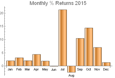
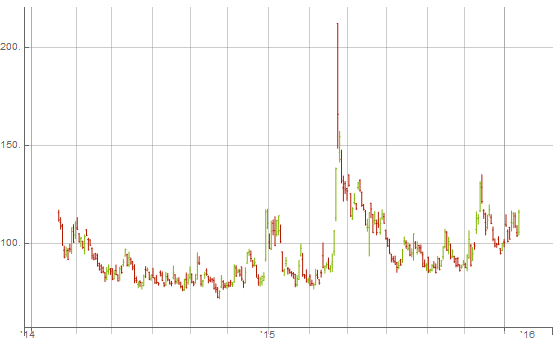
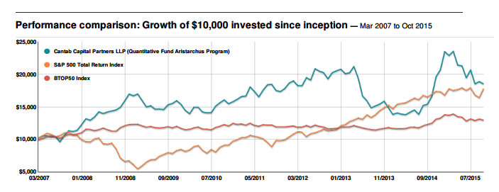
Let’s take a look at how that has worked out in practice:

Fig 1 Fig 2

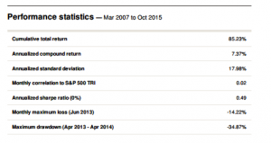
Whatever the fund’s attractions may be, we can at least agree that alpha is not amongst them.  A Sharpe ratio of < 0.5 (I calculate to be nearer 0.41) is hardly in Renaissance territory, so one imagines that the chief benefit of the product must lie in its liquidity and low market correlation.  Uncorrelated it may be, but an investor in the fund must have extremely deep pockets – and a very strong stomach – to handle the 34% drawdown that the fund suffered in 2013.

Improving the Aristarchus Fund Performance

If we make the assumption that an investment in this product is warranted in the first place, what can be done to improve its performance characteristics?  We’ll look at that question from two different perspectives – the investor’s and the manager’s.

Firstly, from the investor’s perspective, there are relatively few options available to enhance the fund’s contribution, other than through diversification.  One other possibility available to the investor, however, is to develop a program for dynamic capital allocation.  This requires the manager to be open to allowing significant changes in the amount of capital to be allocated from month to month, or quarter to quarter, but in a liquid product like Aristarchus some measure of flexibility ought to be feasible.

SSALGOTRADING AD

An analysis of the fund’s performance indicates the presence of a strong dependency in the returns process.  This is not at all unusual.  Often investment strategies have a tendency to mean-revert: a negative dependency in which periods of poor performance tend to be followed by positive performance, and vice versa.  CTA strategies such as Aristarchus tend to be trend-following, and this can induce positive dependency in the strategy returns process, in which positive months tend to follow earlier positive months, while losing months tend to be followed by further losses.  This is the pattern we find here.

Consequently, rather than maintaining a constant capital allocation, an investor would do better to allocate capital dynamically, increasing the amount of capital after a positive period, while decreasing the allocation after a period of losses.  Let’s consider a variation of this allocation plan, in which the amount of allocated capital is increased by 70% when the last monthly equity value exceeds the quarterly moving average, while the allocation is reduced to zero when the last month’s equity falls below the average.  A dynamic capital allocation plan as simple as this appears to produce a significant improvement in the overall performance of the investment:

Fig 4

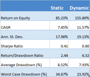
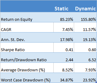
The slight increase in annual volatility in the returns produced by the dynamic capital allocation model is more than offset by the 412bp improvement in the CAGR. Consequently, the Sharpe Ratio improves from o.41 to 0.60.

Nor is this by any means the entire story: the dynamic model produces lower average drawdowns (7.93% vs. 8.52%) and, more importantly, reduces the maximum drawdown over the life of the fund from a painful 34.87% to more palatable 23.92%.

The much-improved risk profile of the dynamic allocation scheme is reflected in the Return/Drawdown Ratio, which rises from 2.44 to 6.52.

Note, too, that the average level of capital allocated in the dynamic scheme is very slightly less than the original static allocation.  In other words, the dynamic allocation technique results in a more efficient use of capital, while at the same time producing a higher rate of risk-adjusted return and enhancing the overall risk characteristics of the strategy.

Improving Fund Performance Using a Meta-Strategy

So much for the investor.  What could the manager to do improve the strategy performance?  Of course, there is nothing in principle to prevent the manager from also adopting a dynamic approach to capital allocation, although his investment mandate may require him to be fully invested at all times.

Assuming for the moment that this approach is not available to the manager, he can instead look into the possibilities for developing a meta-strategy.    As I explained in my earlier post on the topic:

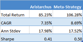
A meta-strategy is a trading system that trades trading systems.  The idea is to develop a strategy that will make sensible decisions about when to trade a specific system, in a way that yields superior performance compared to simply following the underlying trading system.

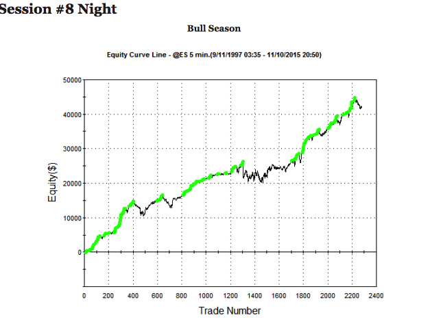
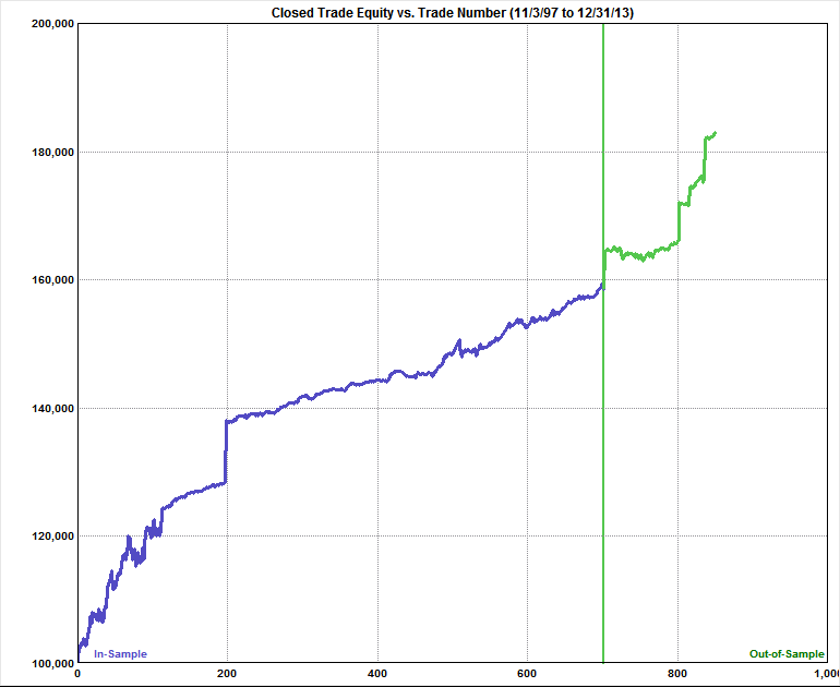
It turns out to be quite straightforward to develop such a meta-strategy, using a combination of stop-loss limits and profit targets to decide when to turn the strategy on or off.  In so doing, the manager is able to avoid some periods of negative performance, producing a significant uplift in the overall risk-adjusted return:

Fig 5

Conclusion

Meta-strategies and dynamic capital allocation schemes can enable the investor and the investment manager to improve the performance characteristics of their investment and investment strategy, by increasing returns, reducing volatility and the propensity of the strategy to produce substantial drawdowns.

We have demonstrated how these approaches can be applied successfully to Cantab’s Aristarchus quantitative fund, producing substantial gains in risk adjusted performance and reductions in the average and maximum drawdowns produced over the life of the fund.