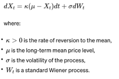
Consider a financial asset whose price, Xt, follows a mean-reverting stochastic process. A common model for mean reversion is the Ornstein-Uhlenbeck (OU) process, defined by the stochastic differential equation (SDE):
Objective
The trader aims to maximize the expected cumulative profit from trading this asset over a finite horizon, subject to transaction costs. The trader’s control is the rate of buying or selling the asset, denoted by ut, at time t.
Hamilton-Jacobi-Bellman (HJB) Equation
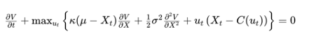
To find the optimal trading strategy, we frame this as a stochastic control problem. The value function,V(t,Xt), represents the maximum expected profit from time t to the end of the trading horizon, given the current price level Xt. The HJB equation for this problem is:
where C(ut) represents the cost of trading, which can depend on the rate of trading ut. The term ut(Xt−C(ut)) captures the profit from trading, adjusted for transaction costs.
Solution Approach
Boundary and Terminal Conditions: Specify terminal conditions for V(T,XT), where T is the end of the trading horizon, and boundary conditions for V(t,Xt) based on the problem setup.
Solve the HJB Equation: The solution involves finding the function V(t,Xt) and the control policy ut∗ that maximizes the HJB equation. This typically requires numerical methods, especially for complex cost functions or when closed-form solutions are not feasible.
Interpret the Optimal Policy: The optimal control ut∗ derived from solving the HJB equation indicates the optimal rate of trading (buying or selling) at any time t and price level Xt, considering the mean-reverting nature of the price and the impact of transaction costs.
Key Insights
No-Trade Zones: The presence of transaction costs often leads to the creation of no-trade zones in the optimal policy, where the expected benefit from trading does not outweigh the costs.
Mean-Reversion Exploitation: The optimal strategy exploits mean reversion by adjusting the trading rate based on the deviation of the current price from the mean level, μ.
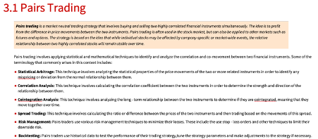
The Lipton & Lopez de Marcos Paper
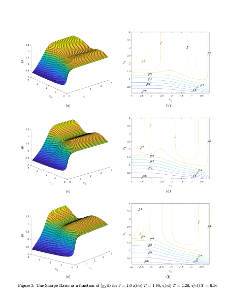
“A Closed-form Solution for Optimal Mean-reverting Trading Strategies” contributes significantly to the literature on optimal trading strategies for mean-reverting instruments. The paper focuses on deriving optimal trading strategies that maximize the Sharpe Ratio by solving the Hamilton-Jacobi-Bellman equation associated with the problem. It outlines a method that relies on solving a Fredholm integral equation to determine the optimal trading levels, taking into account transaction costs.
The paper begins by discussing the relevance of mean-reverting trading strategies across various markets, particularly emphasizing the energy market’s suitability for such strategies. It acknowledges the practical challenges and limitations of previous analytical results, mainly asymptotic and applicable to perpetual trading strategies, and highlights the novelty of addressing finite maturity strategies.
A key contribution of the paper is the development of an explicit formula for the Sharpe ratio in terms of stop-loss and take-profit levels, which allows traders to deploy tactical execution algorithms for optimal strategy performance under different market regimes. The methodology involves calibrating the Ornstein-Uhlenbeck process to market prices and optimizing the Sharpe ratio with respect to the defined levels. The authors present numerical results that illustrate the Sharpe ratio as a function of these levels for various parameters and discuss the implications of their findings for liquidity providers and statistical arbitrage traders.
The paper also reviews traditional approaches to similar problems, including the use of renewal theory and linear transaction costs, and compares these with its analytical framework. It concludes that its method provides a valuable tool for liquidity providers and traders to optimally execute their strategies, with practical applications beyond theoretical interest.
The authors use the path integral method to understand the behavior of their solutions, providing an alternative treatment to linear transaction costs that results in a determination of critical boundaries for trading. This approach is distinct in its use of direct solving methods for the Fredholm equation and adjusting the trading thresholds through a numerical method until a matching condition is met.
This research not only advances the understanding of optimal trading rules for mean-reverting strategies but also offers practical guidance for traders and liquidity providers in implementing these strategies effectively.
Market timing has a very bad press and for good reason: the inherent randomness of markets makes reliable forecasting virtually impossible. So why even bother to write about it? The answer is, because market timing has been mischaracterized and misunderstood. It isn’t about forecasting. If fact, with notable exceptions, most of trading isn’t about forecasting. It’s about conditional expectations.
Conditional expectations refer to the expected value of a random variable (such as future stock returns) given certain known information or conditions.
In the context of trading and market timing, it means that rather than attempting to forecast absolute price levels, we base our expectations for future returns on current observable market conditions.
For example, let’s say historical data shows that when the market has declined a certain percentage from its recent highs (condition), forward returns over the next several days tend to be positive on average (expectation). A trading strategy could use this information to buy the dip when that condition is met, not because it is predicting that the market will rally, but because history suggests a favorable risk/reward ratio for that trade under those specific circumstances.
The key insight is that by focusing on conditional expectations, we don’t need to make absolute predictions about where the market is heading. We simply assess whether the present conditions have historically been associated with positive expected returns, and use that probabilistic edge to inform our trading decisions.
This is a more nuanced and realistic approach than binary forecasting, as it acknowledges the inherent uncertainty of markets while still allowing us to make intelligent, data-driven decisions. By aligning our trades with conditional expectations, we can put the odds in our favor without needing a crystal ball.
So, when a market timing algorithm suggests buying the market, it isn’t making a forecast about what the market is going to do next. Rather, what it is saying is, if the market behaves like this then, on past experience, the following trade is likely to be profitable. That is a very different thing from forecasting the market.
A good example of a simple market-timing algorithm is “buying the dips”. It’s so simple that you don’t need a computer algorithm to do it. But a computer algorithm helps by determining what comprises a dip and the level at which profits should be taken.
An Effective Market Timing Strategy
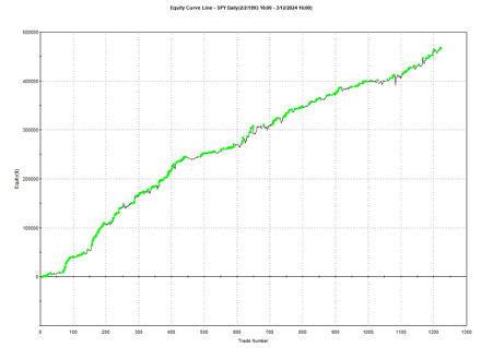
One of my favorites market timing strategies is the following algorithm, which I originally developed to trade the SPY ETF. The equity curve from inception of the ETF in 1993 looks like this:
The algorithm combines a few simple technical indicators to determine what constitutes a dip and the level at which profits should be taken. The entry and exit orders are also very straightforward, buying and selling at the market open, which can be achieved by participating in the opening auction. This is very convenient: a signal is generated after the close on day 1 and is then executed as a MOA (market opening auction) order in the opening auction on day 2. The opening auction is by no means the most liquid period of the trading session, but in an ETF like SPY the volumes are such that the market impact is likely to be negligible for the great majority of investors. This is not something you would attempt to do in an illiquid small-cap stock, however, where entries and exits are more reliably handled using a VWAP algorithm; but for any liquid ETF or large-cap stock the opening auction will typically be fine.
Adapting the Strategy to Other Assets and Markets
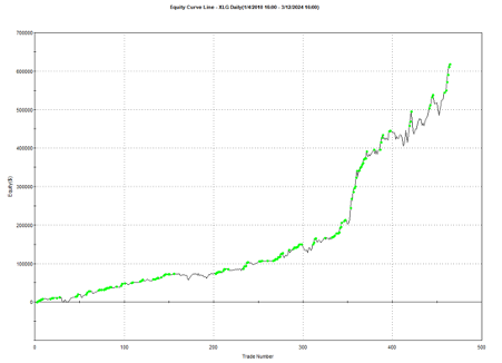
Another aspect that gives me confidence in the algorithm is that it generalizes well to other assets and even other markets. Here, for example, is the equity curve for the exact same algorithm implemented in the XLG ETF in the period from 2010:
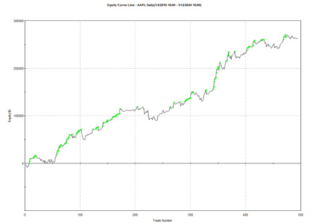
And here is the equity curve for the same strategy (with the same parameters) in AAPL, over the same period:
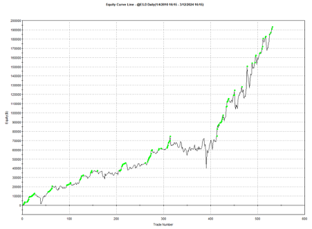
Remarkably, the strategy also works in E-mini futures too, which is highly unusual: typically the market dynamics of the futures market are so different from the spot market that strategies don’t transfer well. But in this case, it simply works:
Understanding Why the Strategy Works
The reason the strategy is effective is due to the upward drift in equities and related derivatives. If you tried to apply a similar strategy to energy or currency markets, it would fail. The strategy’s “secret sauce” is the combination of indicators it uses to determine the short-term low in the ETF that constitutes a good buying opportunity, and then figure out the right level at which to sell.
Does the algorithm always work? If by that you mean “is every trade profitable?” the answer is no. Around 61% of trades are profitable, so there are many instances where trades are closed at a loss. But the net impact of using the market-timing algorithm is very positive, when compared to the buy-and-hold benchmark, as we shall see shortly.
Because the underlying thesis is so simple (i.e. equity markets have positive drift), we can say something about the long-term prospects for the strategy. Equity markets haven’t changed their fundamental tendency to appreciate over the 31-year period from inception of the SPY ETF in 1993, which is why the strategy has performed well throughout that time. Could one envisage market conditions in which the strategy will perform poorly? Yes – any prolonged period of flat to downward trending prices in equities will result in poor performance. But we haven’t seen those conditions since the early 1970’s and, arguably, they are unlikely to return, since the fundamental change brought about by abandonment of the gold standard in 1973.
The abandonment of the gold standard and the subsequent shift to fiat currencies has given central banks, particularly the U.S. Federal Reserve, unprecedented power to expand the money supply and support asset prices during times of crisis. This ‘Fed Put’ has been a major factor underpinning the multi-decade bull market in stocks.
In addition, the increasing dominance of the U.S. as the world’s primary economic and military superpower since the end of the Cold War has made U.S. financial assets a uniquely attractive destination for global capital, creating sustained demand for U.S. equities.
Technological innovation, particularly with respect to the internet and advances in computing, has also unleashed a wave of productivity and wealth creation that has disproportionately benefited the corporate sector and equity holders. This trend shows no signs of abating and may even be accelerating with the advent of artificial intelligence.
While risks certainly remain and occasional cyclical bear markets are inevitable, the combination of accommodative monetary policy, the U.S.’s global hegemony, and technological progress create a powerful set of economic forces that are likely to continue propelling equity prices higher over the long-term, albeit with significant volatility along the way.Strategy Performance in Bear Markets
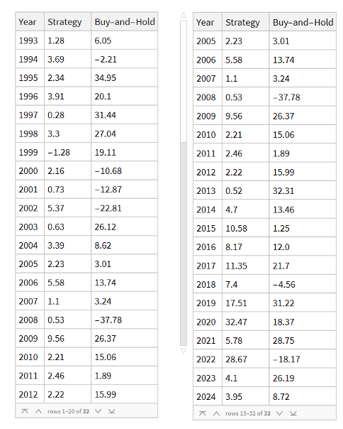
Note that the conditions I am referring to are something unlike anything we have seen in the last 50 years, not just a (serious) market pullback. If we look at the returns in the period from 2000-2002, for example, we see that the strategy held up very well, out-performing the benchmark by 54% over the three-year period of the market crash. Likewise, in 2008 credit crisis, the strategy was able to eke out a small gain, beating the benchmark by over 38%. In fact, the strategy is positive in all but one of the 31 years from inception.
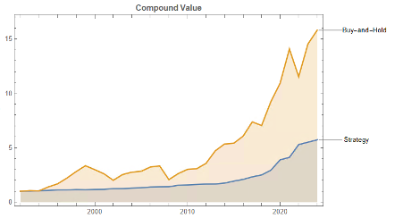
Comparing Performance to Buy-and-Hold
Let’s take a look at the compound returns from the strategy vs. the buy-and-hold benchmark:
At first sight, it appears that the benchmark significantly out-performs the strategy, albeit suffering from much larger drawdowns. But that doesn’t give an accurate picture of relative performance. To see why, let’s look at the overall performance characteristics:
Now we see that, while the strategy CAGR is 3.50% below the buy-and-hold return, its annual volatility is less than half that of the benchmark, giving the strategy a superior Sharpe Ratio.
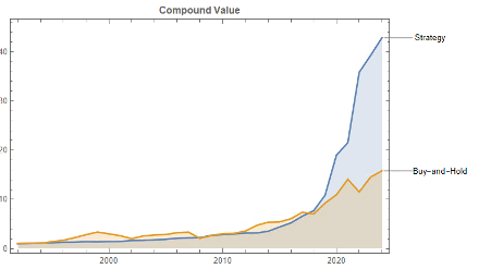
Leveraging the Strategy to Enhance Risk-Adjusted Returns
To make a valid comparison between the strategy and its benchmark we therefore need to equalize the annual volatility of both, and we can achieve this by leveraging the strategy by a factor of approximately 2.32. When we do that, we obtain the following results:
Now that the strategy and benchmark volatilities have been approximately equalized through leverage, we see that the strategy substantially outperforms buy-and-hold by around 355 basis points per year and with far smaller drawdowns.
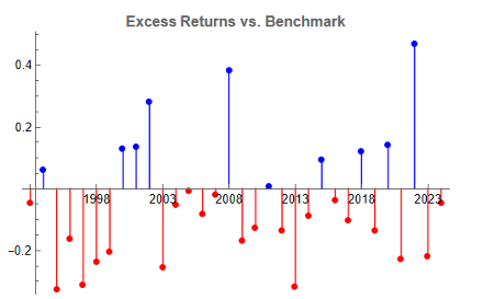
In general, we see that the strategy outperformed the benchmark in fewer than 50% of annual periods since 1993. However, the size of the outperformance in years when it beat the benchmark was frequently very substantial:
Conclusion
Market timing can work. To understand why, we need to stop thinking in terms of forecasting and think instead about conditional returns. When we do that, we arrive at the insight that market timing works because it relies on the positive drift in equity markets, which has been one of the central features of that market over the last 50 years and is likely to remain so in the foreseeable future. We have confidence in that prediction, because we understand the economic factors that have continued to drive the upward drift in equities over the last half-century.
After that, it is simply a question of the mechanics – how to time the entries and exits. This article describes just one approach amongst a great number of possibilities.
One of the many benefits of market timing is that it has a tendency to side-step the worst market conditions and can produce positive returns even in the most hostile environments: periods such as 2000-2002 and 2008, for example, as we have seen.
Finally, don’t forget that, as we are sitting out of the market approximately 40% of the time our overall risk is much lower – less than half that of the benchmark. So, we can afford to leverage our positions without taking on more overall risk than when we buy and hold. This clearly demonstrates the ability of the strategy to produce higher rates of risk-adjusted return.
Financial modeling has long sought to develop frameworks that accurately capture the complex dynamics of asset prices. Traditional models often focus on either momentum or mean reversion effects, struggling to incorporate both simultaneously. In this blog post, we introduce a two-factor model that aims to address this issue by integrating both momentum and mean reversion effects within the stochastic processes governing stock prices.
The Motivation Behind the Two-Factor Model:
The development of the two-factor model is motivated by the empirical observation that financial markets exhibit periods of persistent trends (momentum) and reversion to historical means or intrinsic values (mean reversion). Capturing both effects within a single framework has been a challenge in financial econometrics. The proposed model seeks to tackle this challenge by incorporating momentum and mean reversion effects within a unified framework.
The Building Blocks of the Two-Factor Model:
The two-factor model consists of two main components: a drift factor and a mean-reverting factor. The drift factor, denoted as d μ(t), represents the long-term trend or momentum of a stock’s price. It incorporates a constant drift parameter θ, reflecting the underlying direction driven by broader market forces or fundamental changes. The mean-reverting factor, denoted as d θt, captures the short-term deviations from the drift. It is characterized by a mean-reversion speed κ, which determines the rate at which prices revert to their long-term equilibrium following temporary fluctuations. These factors are influenced by their respective volatilities (σμ, σθ) and driven by correlated Wiener processes, allowing the model to reflect the interaction between momentum and mean reversion observed in markets
Empirical Application and Parameter Estimation:
To demonstrate the model’s application, the research applies the two-factor framework to daily returns data of Coca-Cola (KO) and PepsiCo (PEP) over a twenty-year period. This empirical analysis explores the model’s potential for informing pairs trading strategies. The parameter estimation process employs a maximum likelihood estimation (MLE) technique, adapted to handle the specifics of fitting a two-factor model to real-world data. This approach aims to ensure accuracy and adaptability, enabling the model to capture the evolving dynamics of the market.
Implications for Financial Modeling and Trading Strategies:
The introduction of the two-factor model contributes to the field of quantitative finance by providing a framework that incorporates both momentum and mean reversion effects. This approach can lead to a more comprehensive understanding of asset price dynamics, potentially benefiting risk management, asset allocation, and the development of trading strategies. The model’s insights may be particularly relevant for pairs trading, where identifying relative mispricings between related assets is important.
Conclusion:
The two-factor model presented in this blog post offers a new approach to financial modeling by integrating momentum and mean reversion effects. The model’s empirical application to Coca-Cola and PepsiCo demonstrates its potential for informing trading strategies. As quantitative finance continues to evolve, the two-factor model may prove to be a useful tool for researchers, practitioners, and investors seeking to understand the dynamics of financial markets.
High-frequency statistical arbitrage leverages sophisticated quantitative models and cutting-edge technology to exploit fleeting inefficiencies in global markets. Pioneered by hedge funds and proprietary trading firms over the last decade, the strategy identifies and capitalizes on sub-second price discrepancies across assets ranging from public equities to foreign exchange.
At its core, statistical arbitrage aims to predict short-term price movements based on probability theory and historical relationships. When implemented at high frequencies—microseconds or milliseconds—the quantitative models uncover trading opportunities unavailable to human traders. The predictive signals are then executable via automated, low-latency infrastructure.
These strategies thrive on speed. By getting pricing data faster, determining anomalies faster, and executing orders faster than the rest of the market, you expand the momentary windows to trade profitably.
Seminal papers have delved into the mathematical and technical nuances underpinning high-frequency statistical arbitrage. Zhaodong Zhong and Jian Wang’s 2014 paper develops stochastic models to quantify how market microstructure and randomness influence high-frequency trading outcomes. Samuel Wong’s 2018 research explores adapting statistical arbitrage for the nascent cryptocurrency markets.
Yet maximizing the strategy’s profitability poses an ongoing challenge. Changing market dynamics necessitate regular algorithm tweaking and infrastructure upgrades. It’s an arms race for lower latency and better predictive signals. Any edge gained disappears quickly as new firms implement similar systems. Regulatory attention also persists due to concerns over unintended impacts on market stability.
Nonetheless, high-frequency statistical arbitrage retains a crucial role for leading quant funds. Ongoing advances in machine learning, cloud computing, and execution technology promise to further empower the strategy. Though the competitive landscape grows more challenging, the cutting edge continues advancing profitably. Where human perception fails, automated high-frequency strategies recognize and seize value.
Implementing an Intraday Statistical Arbitrage Model
While HFT infrastructure and know-how are beyond the reach of most traders, it is possible to conceive of a system for pairs trading at moderate frequency, say 1-minute intervals.
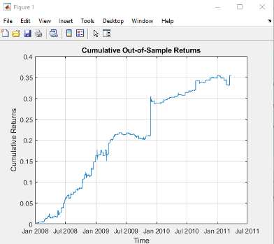
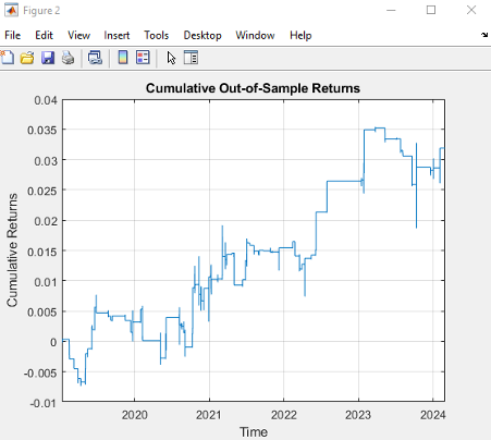
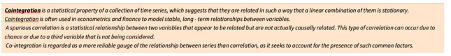
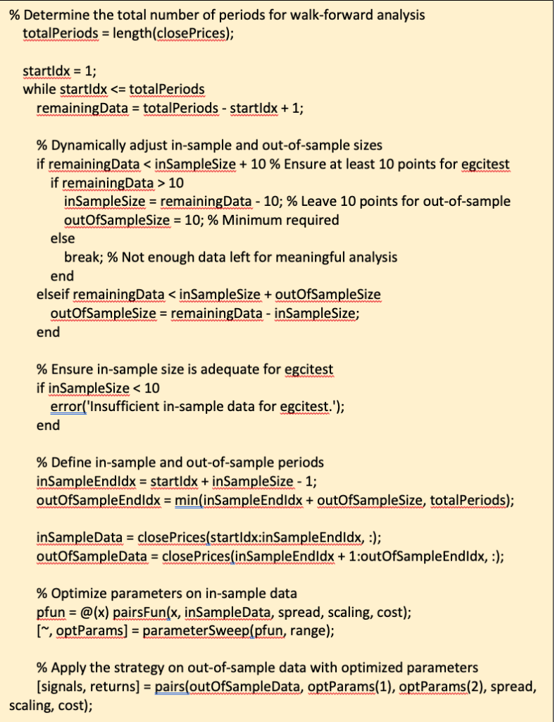
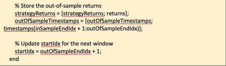
We illustrate the approach with an algorithm that was originally showcased by Mathworks some years ago (but which has since slipped off the radar and is no longer available to download). I’ve amended the code to improve its efficiency, but the core idea remains the same: we conduct a rolling backtest in which data on a pair of assets, in this case spot prices of Brent Crude (LCO) and West Texas Intermediate (WTI), is subdivided into in-sample and out-of-sample periods of varying lengths. We seek to identify windows in which the price series are cointegrated in the sense of Engle-Granger and then apply the regression parameters to take long and short positions in the pair during the corresponding out-of-sample period. The idea is to trade only when there is compelling evidence of cointegration between the two series and to avoid trading at other times.
The critical part of the walk-forward analysis code is as shown below. Note we are using a function parametersweep to conduct a grid search across a range of in-sample dataset sizes to determine if the series are cointegrated (according to the Engle-Granger test) in that sub-period and, if so, determine the position size according to the regression parameters. The optimal in-sample parameters are then applied in the out-of-sample period and the performance results are recorded.
Here we are making use of Matlab’s parallelization capabilities, which work seamlessly to spread the processing load across available CPUs, handling the distribution of variables, function definitions and dependencies with ease. My experience with trying to parallelize Python, by contrast, is often a frustrating one that frequently fails at the first several attempts.
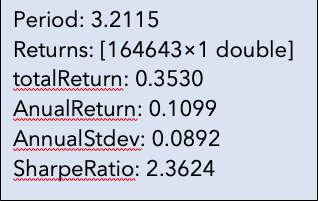
The results appear promising; however, the data is out-of-date, comes from a source that can be less than 100% reliable and may represent price quotes rather than traded prices. If we switch to 1-minute traded prices in a pair of stocks such as PEP and KO that are known to be cointegrated over long horizons, the outcome is very different:
Conclusion
High-frequency statistical arbitrage represents the convergence of cutting-edge technology and quantitative modeling to uncover fleeting trading advantages invisible to human market participants. This strategy has proven profitable for sophisticated hedge funds and prop shops, but also raises broader questions around fairness, regulation, and the future of finance.
However, the competitive edge gained from high-frequency strategies diminishes quickly as the technology diffuses across the industry. Firms must run faster just to stand still.
Continued advancement in machine learning, cloud computing, and execution infrastructure promises to expand the frontier. But practitioners and policymakers alike share responsibility for ensuring market integrity and stability amidst this technology arms race.
In conclusion, high-frequency statistical arbitrage remains essential to many leading quantitative firms, with the competitive landscape growing ever more challenging. Realizing the potential of emerging innovations, while promoting healthy markets that benefit all participants, will require both vision and wisdom. The path ahead lies between cooperation and competition, ethics and incentives. By bridging these domains, high-frequency strategies can contribute positively to financial evolution while capturing sustainable edge.
References:
Zhong, Zhaodong, and Jian Wang. “High-Frequency Trading and Probability Theory.” (2014).
Wong, Samuel S. Y. “A High-Frequency Algorithmic Trading Strategy for Cryptocurrency.” (2018).
Glossary
For those unfamiliar with the topic of statistical arbitrage and its commonly used terms and concepts, check out my book Equity Analytics, which covers the subject matter in considerable detail.
In a previous article I made a detailed comparison of Mathematica and Python and tried to identify areas where the former excels. Despite the many advantages of the Python technology stack, I was able to pinpoint a few areas in which I think Mathematica holds the upper hand. Whether those are sufficient to warrant the investment of time and money required to master the Wolfram Language is another matter, which the user must decide for himself.
In this comparison between Matlab and Python I won’t reiterate the strengths of the Python that make it the programming language of choice for so many developers. Let me instead focus on some of the key aspects of Matlab where I think the Mathworks product outshines its rival.
Matlab is designed for numerical computing, while Python is a general-purpose programming language that has become a major tool for scientific computing through libraries like NumPy, SciPy, and Matplotlib.
The key advantages of Matlab relative to Python, as I see them, are as follows:
Integrated Development Environment (IDE):
Matlab comes with a feature-rich IDE that is tailored for mathematical and engineering workflows. This includes tools for debugging, data visualization, GUI creation, and managing workspace variables. The Matlab IDE is specifically designed to streamline the development of mathematical and engineering applications.
Advanced Toolboxes:
Matlab offers a wide range of specialized toolboxes for different applications, including signal processing, control systems, neural networks, image processing, and many others. These toolboxes are professionally developed, rigorously tested, and regularly updated, providing a comprehensive suite of algorithms and functions for specific domains. With its vast ecosystem of scientific libraries Python has caught up with Matlab in recent years, and even overtaken it in some areas, but Matlab’s toolboxes are tried and battle-tested technologies that are used by millions of users in state-of-the-art applications.
Simulink:
Matlab provides Simulink, a platform for Model-Based Design for dynamic and embedded systems. Simulink is a graphical programming environment for modeling, simulating, and analyzing multidomain dynamical systems. This is particularly useful in engineering applications where system modeling and simulation are crucial.
Built-in Support for Matrix Operations:
Matlab (Matrix Laboratory) has inherent support for matrix operations and linear algebra, making it highly efficient for tasks that involve complex mathematical computations.
Performance:
Matlab is optimized for operations involving matrices and vectors, which are central to engineering and scientific computations. For certain numerical tasks, Matlab’s performance is superior due to its highly optimized code and ability to handle parallel computing and GPU acceleration effectively.
Matlab’s speed has further accelerated over the last decade due to just-in-time compilation. This feature automatically compiles Matlab’s interpreted code into machine code at runtime, which speeds up execution, especially in loops and computationally intensive tasks. The JIT compilation process is entirely transparent to the user, requiring no modifications to the code or the development process. Python itself is an interpreted language and does not include JIT compilation in its standard implementation (CPython). However, JIT compilation can be introduced through third-party libraries or alternative Python implementations, such as Numba or PyPy.
Testing and Debugging:
Both Matlab and Python are equipped with robust testing and debugging tools that cater to their specific user bases. Matlab’s tools are tightly integrated into its IDE and are particularly tailored for numerical computing and engineering tasks. I would regard them as the industry standard in terms of features, ease of use and helpfulness. In contrast, Python’s testing and debugging ecosystem is more diverse, with multiple options available for different tasks, including third-party libraries that extend its capabilities.
Documentation and Support:
Matlab’s documentation is extensive, well-organized, and includes examples for a wide range of functions and toolboxes. Additionally, MathWorks provides excellent support services, including technical support and community forums, which can be particularly valuable for complex or specialized projects.
Conclusion
While Python has gained significant popularity in scientific computing, data science, and machine learning due to its open-source nature and the vast ecosystem of libraries, Matlab holds strong advantages in numerical computing, engineering applications, and when integrated solutions with robust support and documentation are required.
However, Python offers greater flexibility, scalability and has grown significantly in scientific computing. MATLAB historically had limitations with very large datasets, but recent releases have added features to improve performance with big data. Still, Python likely retains an advantage for extreme scales. The choice depends on the specific use case – for small-scale numerical computing and modeling MATLAB provides an integrated optimized environment while Python excels in general-purpose programming and very large-scale data intensive applications. However, both continue to evolve impressive capabilities so the lines are blurring. Ultimately data scientists and engineers are best served by being proficient in both languages.
As an avid user of both Python and Wolfram Language for technical computing, I’m often asked how they compare. Python’s strengths as an open-source language are clear:
Ubiquity – With millions of users, Python has become ubiquitous across fields like data science, ML engineering, web development, and scientific research. This massive adoption fuels continuous enhancement of its tools.
Comprehensive capabilities – Python’s expansive ecosystem of 200,000+ libraries spans everything from numerical computing to web frameworks to industrial automation. It is a versatile, widely-supported language for building end-to-end applications.
Approachability – Python’s straightforward syntax, multitude of online resources, and abundance of machine learning libraries like TensorFlow and PyTorch make it highly accessible for new programmers and non-CS domain experts alike.
Interoperability – Python integrates smoothly with everything from SQL and NoSQL databases to enterprise IT environments and microcontrollers like Raspberry Pi. This flexibility enables diverse production deployments.
In summary, Python offers benefits in ubiquity, breadth, approachability, and seamless interoperability with external systems. Together, they show the value of domain-specific and general-purpose languages for tackling modern analytics and engineering challenges.
However, while Python is a versatile, open-source language popular among developers, the Wolfram Language offers some unique advantages:
Powerful Symbolic Capabilities
One of the most powerful aspects of the Wolfram Language is its unparalleled symbolic manipulation abilities for mathematical computation. Operations like symbolic integration, solving equations analytically, theorem proving, model simplification and more are built deeply into the language in a way no other programming language matches. Python can conduct numeric computation and data analysis well, but does not have this domain of symbolic capabilities natively.
For any usage involving abstract mathematical development, derivation of analytical results, or formal proofs, the symbolic nature of the Wolfram Language is a major differentiator.
Wolfram Notebooks
offer notable advantages over Jupyter notebooks in Python:
More visual appeal – The Wolfram notebooks produce beautifully typeset output and publication-ready visualizations by default, whereas Jupyter’s output is more basic.
Greater configurability – Wolfram’s notebooks allow extensive styling, templating, and customization of content for different applications. Jupyter also enables some configuration, but not to the same degree.
Tighter integration – The Wolfram notebooks leverage the language’s underlying functions and capabilities more fluidly since it’s one integrated environment. Jupyter interfaces well with Python but there is still some separation.
Interactivity – Wolfram notebooks support advanced interactivity through Manipulate/Animate and instant visual output.
Overall, while Jupyter notebooks are hugely popular among Python developers and enable great functionality, Wolfram’s notebook solution stands out as more robust, customizable, and visually polished. The tight integration with the Wolfram Language and computational capabilities augments interactive analysis in a way Jupyter can’t match.
Integrated Knowledge and Data
The Wolfram Language stands out in providing an “integrated knowledge base” that spans from sophisticated algorithms to real-world data across domains. This includes vast curated datasets on topics from architecture to chemistry to finance that can readily feed models and analyses without additional wrangling.
Additionally, the entity store concept allows users to author their own object-based, customizable data repositories. Python’s classes are focused on methods rather than data and while Python offers strong libraries for storing and accessing data, Wolfram facilitates more zero-friction application of real-world knowledge and entity-oriented data storage out-of-the-box. For minimizing time manipulating data or searching for reference algorithms before modeling, Wolfram Language excels.
The entity store in particular enables a very natural object/entity-based programming style that can integrate smoothly with Wolfram’s class system and its underlying symbolic capabilities. This unique data representation system differentiation is a key strength (for example, see the Equities Entity Store).
Interactivity and Prototyping
The Wolfram Language excels in hands-on analysis and rapid iteration thanks to its line-by-line execution and built-in Manipulate/Animate functions for customizable graphics, animations and interactive simulations. Python does allow some interactivity in Jupyter notebooks, but does not match Wolfram’s capabilities for creating interactive visualizations on-the-fly. This makes Wolfram Language uniquely well-suited for highly iterative, prototyping tasks that involve visual output. If ease of exploration and fluid development is a priority, the Wolfram Language has clear strengths.
Seamless Parallelization
The Wolfram Language has seamless built-in parallelization capabilities that allow code to efficiently utilize multi-core systems without the developer needing to directly manage threads or processes. Python can achieve parallelism through libraries, but the developer bears responsibility for managing dependencies and avoiding conflicts. Similarly, the Wolfram Language directly interfaces with Nvidia GPUs out-of-the-box for high performance numerical code with minimal extra effort. Thus, for users focused on computational speedup, Wolfram simplifies parallelization and GPU integration in very useful ways.
Python libraries like TensorFlow and PyTorch do hide GPU complexities well for deep learning. But in general, achieving parallel execution in Python places a greater burden on the developer. Wolfram’s approach dramatically lowers the barriers to leveraging multiple cores and GPU power for everyday computations.
Sophisticated Visualization
Creating publication-quality, customized visualizations requires just lines of code in the Wolfram Language, thanks to the built-in graphics capabilities. While Python offers powerful visualization through add-on libraries like Matplotlib, Seaborn, Bokeh, and Plotly, Wolfram’s out-of-the-box solutions may provide greater ease of use. However, from low-level control to interactive web plots, Python’s visualization options are quite extensive despite requiring more setup. Ultimately, for rapid high-level plotting, Wolfram Language has advantageous default capabilities. But Python gives more flexibility and customization options through its ecosystem of graphic libraries.
In summary, while Python offers flexibility and a large user base – advantages in its own right – the Wolfram Language dramatically reduces lines of code and development time. By curating real-world data, algorithms, and visualization in one coherent language and platform, it streamlines and accelerates quantitative work for scientists, analysts, economists and more.
If you do significant data analysis or modeling, I encourage you to try the Wolfram Language and see the difference yourself. It’s been a gamechanger for my productivity.
I’m delighted to introduce my new series of custom-designed AI tools powered by cutting-edge generative technology. With just a click, you can now access a range of intelligent assistants tailored for different tasks.
These AI helpers are the product of fine-tuning powerful models called Generative Pre-trained Transformers (GPTs). I’ve carefully adjusted them to excel at everything from writing to math to coding and beyond.
To try one out, simply click the icon below for the assistant you need. A new world of AI support is now at your fingertips.
As a subscriber to ChatGPT, you can use these GPT-based assistants entirely for free.
I’ll also be expanding the collection as I develop more, so be sure to bookmark this page and sign up for my blog to receive updates and new releases.
Let my growing cast of AI experts supercharge your work and unleash your productivity. The future is here – let them help you take on any task or challenge imaginable. Just click and tell them how they can lend a hand.