Financial modeling has long sought to develop frameworks that accurately capture the complex dynamics of asset prices. Traditional models often focus on either momentum or mean reversion effects, struggling to incorporate both simultaneously. In this blog post, we introduce a two-factor model that aims to address this issue by integrating both momentum and mean reversion effects within the stochastic processes governing stock prices.
The Motivation Behind the Two-Factor Model:
The development of the two-factor model is motivated by the empirical observation that financial markets exhibit periods of persistent trends (momentum) and reversion to historical means or intrinsic values (mean reversion). Capturing both effects within a single framework has been a challenge in financial econometrics. The proposed model seeks to tackle this challenge by incorporating momentum and mean reversion effects within a unified framework.
The Building Blocks of the Two-Factor Model:
The two-factor model consists of two main components: a drift factor and a mean-reverting factor. The drift factor, denoted as d μ(t), represents the long-term trend or momentum of a stock’s price. It incorporates a constant drift parameter θ, reflecting the underlying direction driven by broader market forces or fundamental changes. The mean-reverting factor, denoted as d θt, captures the short-term deviations from the drift. It is characterized by a mean-reversion speed κ, which determines the rate at which prices revert to their long-term equilibrium following temporary fluctuations. These factors are influenced by their respective volatilities (σμ, σθ) and driven by correlated Wiener processes, allowing the model to reflect the interaction between momentum and mean reversion observed in markets
Empirical Application and Parameter Estimation:
To demonstrate the model’s application, the research applies the two-factor framework to daily returns data of Coca-Cola (KO) and PepsiCo (PEP) over a twenty-year period. This empirical analysis explores the model’s potential for informing pairs trading strategies. The parameter estimation process employs a maximum likelihood estimation (MLE) technique, adapted to handle the specifics of fitting a two-factor model to real-world data. This approach aims to ensure accuracy and adaptability, enabling the model to capture the evolving dynamics of the market.
Implications for Financial Modeling and Trading Strategies:
The introduction of the two-factor model contributes to the field of quantitative finance by providing a framework that incorporates both momentum and mean reversion effects. This approach can lead to a more comprehensive understanding of asset price dynamics, potentially benefiting risk management, asset allocation, and the development of trading strategies. The model’s insights may be particularly relevant for pairs trading, where identifying relative mispricings between related assets is important.
Conclusion:
The two-factor model presented in this blog post offers a new approach to financial modeling by integrating momentum and mean reversion effects. The model’s empirical application to Coca-Cola and PepsiCo demonstrates its potential for informing trading strategies. As quantitative finance continues to evolve, the two-factor model may prove to be a useful tool for researchers, practitioners, and investors seeking to understand the dynamics of financial markets.
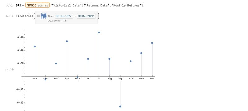
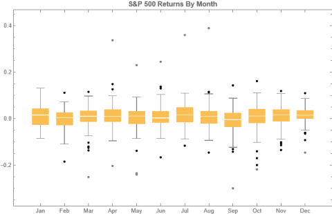
To amplify Valérie Noël‘s post a little, we can use the Equities Entity Store (https://lnkd.in/epg-5wwM) to extract returns for the S&P500 index for (almost) the last century and compute the average return by month, as follows.
July is shown to be (by far) the most positive month for the index, with an average return of +1.67%, in stark contrast to the month of Sept. in which the index has experienced an average negative return of -1.15%.
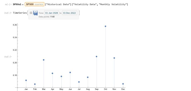
Continuing the analysis a little further, we can again use the the Equities Entity Store (https://lnkd.in/epg-5wwM) to extract estimated average volatility for the S&P500 by calendar month since 1927:
As you can see, July is not only the month with highest average monthly return, but also has amongst the lowest levels of volatility, on average.
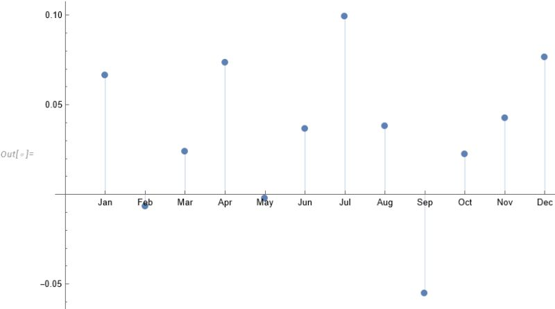
Consequently, risk-adjusted average rates of return in July far exceed other months of the year.
Conclusion: bears certainly have a case that the market is over-stretched here, but I would urge caution: hold off until end Q3 before shorting this market in significant size.
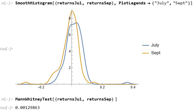
For those market analysts who prefer a little more analytical meat, we can compare the median returns for the #S&P500 Index for the months of July and September using the nonparametric MannWhitney test.
This indicates that there is only a 0.13% probability that the series of returns for the two months are generated from distributions with the same median.
Conclusion: Index performance in July really is much better than in September.
For more analysis along these lines, see my recent book, Equity Analytics:
Generally speaking, one of the major attractions of working in the equities space is that the large number of available securities opens up a much wider range of opportunities for the quantitative researcher than for, say, futures markets. The focus in equities tends to be on portfolio strategies since the scope of the universe permits an unparalleled degree of diversification. Single stock strategies forego such benefit, but they are of interest to the analyst and investor nonetheless: “stock picking” is almost a national pastime, at least for US investors.
Rather than seeking to mitigate stock specific risk through diversification, the stock picker is actively seeking to identify risk opportunities that are unique to a specific stock, and he hopes will yield abnormal returns. These can arise for any number of reasons – mergers and acquisitions, new product development, change in index membership, to name just a few. The hope is that such opportunities may be uncovered by one of several possible means:
Identification of latent, intrinsic value in neglected stocks that has been overlooked by other analysts
The use of alternative types of data that permits new insight in the potential of a specific stock or group of stocks
A novel method of analysis that reveals hitherto hidden potential in a particular stock or group of stocks
One can think of examples of each of these possibilities, but at the same time it has to be admitted that the challenge is very considerable. Firstly, your discovery or methodology would have to be one that has eluded some of the brightest minds in the investment industry. That has happened in the past and will no doubt occur again in future; but the analyst has to have a fairly high regard for his own intellect – or good fortune – to believe that the golden apple will fall into his lap, rather than another’s. Secondly there is the question of the efficient market hypothesis. These days it is fashionable to pour scorn on the EMH, with examples of well-known anomalies often used to justify the opprobrium. But the EMH doesn’t say that markets are 100% efficient, 100% of the time. It says that markets are efficient, on average. This means that there will be times or circumstances in which the market will be efficient and other times and circumstances when it will be relatively inefficient – but you won’t be able to discern which condition the market is in currently. Finally, even if one is successful in identifying such an opportunity, the benefit has to be realizable and economically significant. I can think of several examples of equity strategies that appear to offer the potential to generate alpha, but which turn out to be either unrealizable or economically insignificant after applying transaction costs.
All this is to say that stock picking is one of the most difficult challenges the analyst can undertake. It is also one of the most interesting challenges – and best paid occupations – on Wall Street. So it is unsurprising that for analysts it remains the focus of their research and ambition. In this chapter we will look at some of the ways in which the Equities Entity Store can be used for such purposes and some of the more interesting analytical methods.
Why Technical Analysis Doesn’t Work
Technical Analysis is a very popular approach to analysing stocks. Unfortunately, it is also largely useless, at least if the intention is to uncover potential sources of alpha. The reason is not hard to understand: it relies on applying analytical methods that have been known for decades to widely available public information (price data). There isn’t any source of competitive advantage that might reliably produce abnormal returns. Even the possibility of uncovering a gem amongst the stocks overlooked by other analysts appears increasingly remote these days, as the advent of computerized trading systems has facilitated the application of standard technical analysis tools on an industrial scale. You don’t even need to understand how the indicators work – much less how to program them – in order to apply them to tens of thousands of stocks.
And yet Technical Analysis remains very popular. Why so? The answer, I believe, is because it’s easy to do and can often look very pretty. I will go further and admit that some of the indicators that analysts have devised are extraordinarily creative. But they just don’t work. In fact, I can’t think of another field of human industry that engages so many inventive minds in such a fruitless endeavor.
All this has been clear for some time and yet every year legions of newly minted analysts fling themselves into the task of learning how to apply Technical Analysis to everything from cattle futures to cryptocurrencies. Realistically, the chances of my making any kind of impression on this torrent of pointless hyperactivity are close to zero, but I will give it a go.
A Demonstration
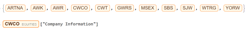
Let’ s begin by picking a stock at random, one I haven’ t look at previously :
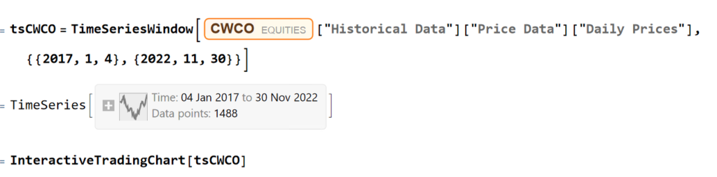
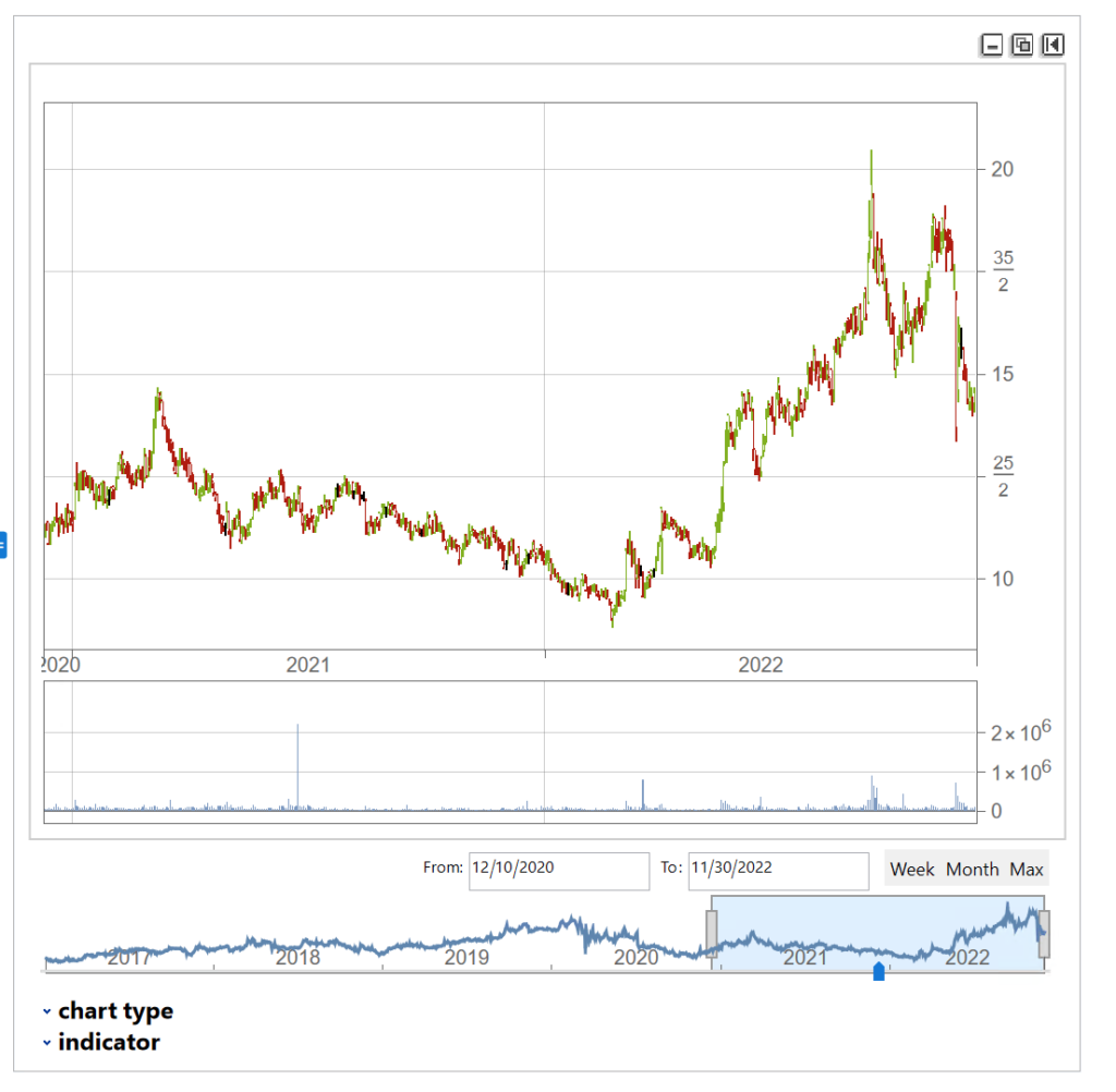
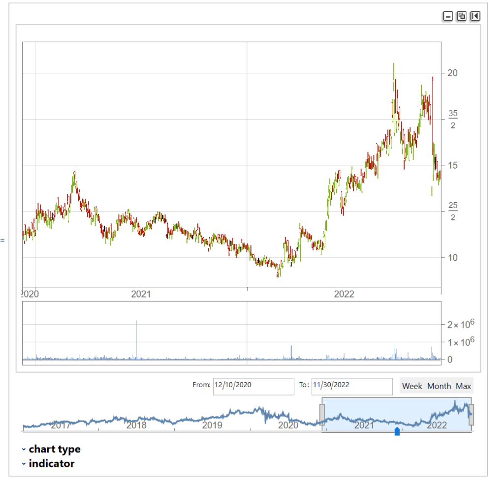
We’ll extract a daily price series from 2017 to 2022 and plot an interactive trading chart, to which we can add moving averages, or any number of other technical indicators, as we wish:
The chart shows several different types of pattern that are well-known to technical analysis, including trends, continuation patterns, gaps, double tops, etc
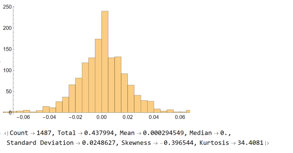
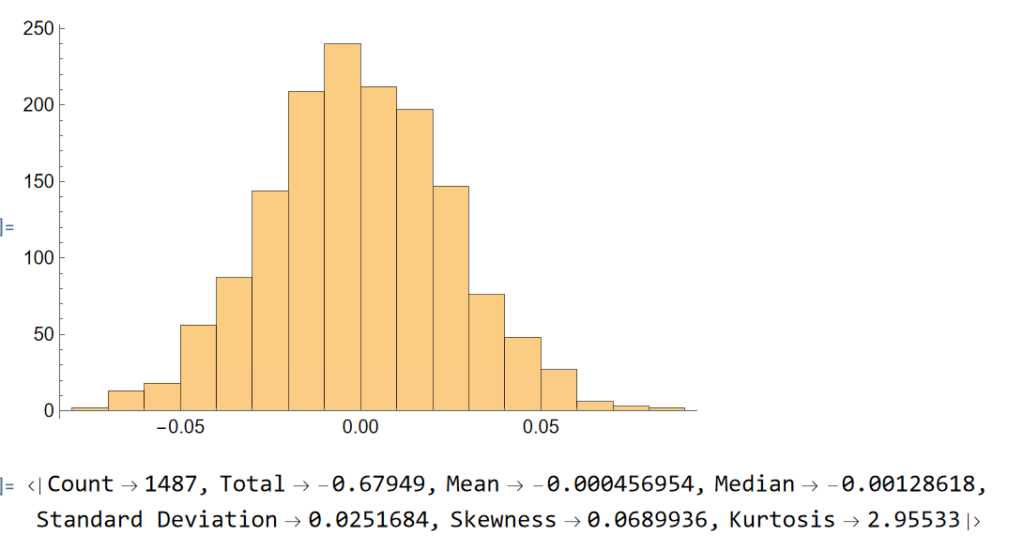
Next, we will generate a series of random returns, drawn from a Gaussian distribution with the same mean and standard deviation as the empirical returns series:
Clearly, the distribution of the generated returns differs from the distribution of empirical returns, but that doesn’t matter: all that counts is that we can agree that the generated returns, which represent the changes in (log) prices from one day to the next, are completely random. Consequently, knowing the random returns, or prices, at time t = 1, 2, . . . , (t-1) in no way enables you to forecast the return , or price, at time t.
Now let’ s generate a series of synthetic prices and time series, using the synthetic returns to calculate the prices for each period:
The synthetic time series is very similar to the original and displays many of the same characteristics, including classical patterns that are immediately comprehensible to a technical analyst, such as gaps, reversals , double tops, etc.
But the two time series, although similar, are not identical:
tsCWCO===tsSynthetic

False
We knew this already, of course, because we used randomly generated returns to create the synthetic price series. What this means is that, unlike for the real price series, in the case of the synthetic price series we know for certain that the movement in prices from one period to the next is entirely random. So if prices continue in an upward trend after a gap, or decline after a double top formation appears on the chart of the synthetic series, that happens entirely by random chance, not in response to a pattern flagged by the technical indicator. If we had generated a different set of random returns, we could just as easily have produced a synthetic price series in which prices reversed after a gap up, or continued higher after a double-top formation. Critics of Technical Analysis do not claim that patterns such as gaps, head and shoulders , etc., do not exist – they clearly do. Rather, we say that such patterns are naturally occurring phenomena that will arise even in a series known to be completely random and hence can have no economic significance.
The point is not to say that technical signals never work: sometimes they do and sometimes they don’t. Rather, the point is that, in any given situation, you will be unable to tell whether the signal is going to work this time, or not – because price changes are dominated by random variation.
You can make money in the markets using technical analysis, just as you can by picking stocks at random, throwing darts at a dartboard, or tossing a coin to decide which to buy or sell – i.e. by dumb luck. But you can’t reliably make money this way.
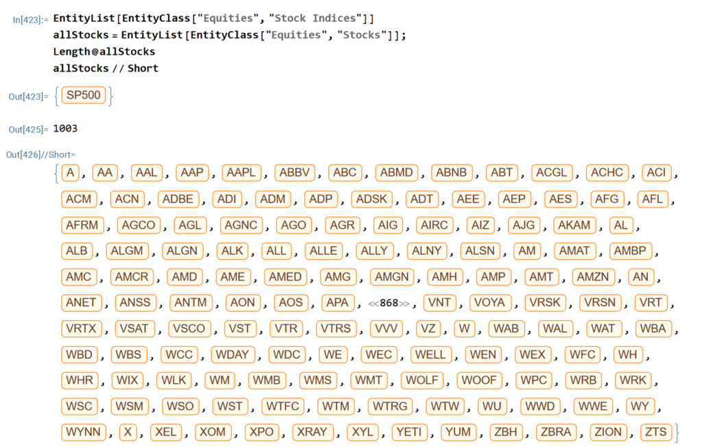
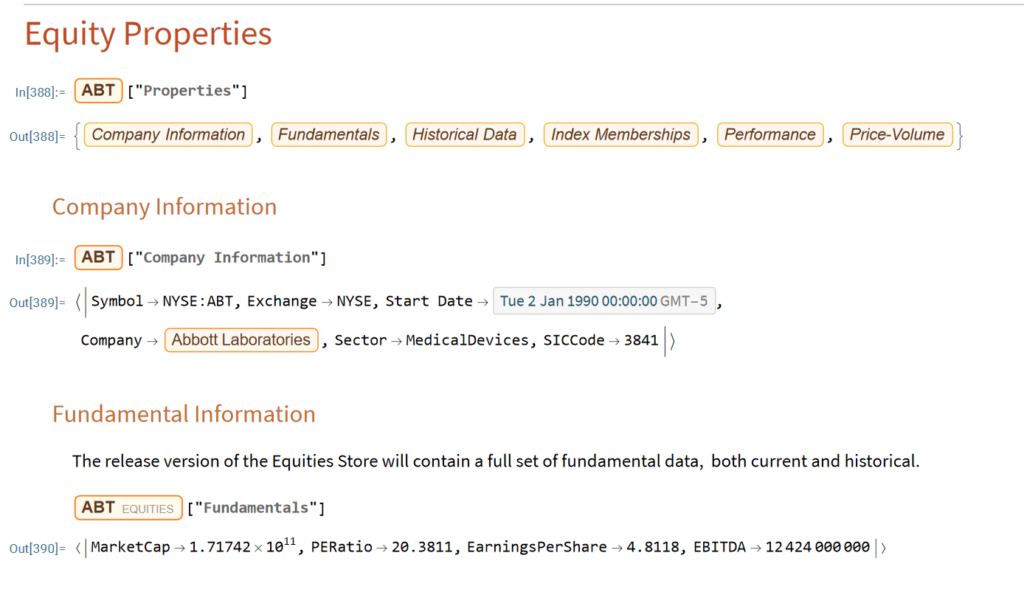
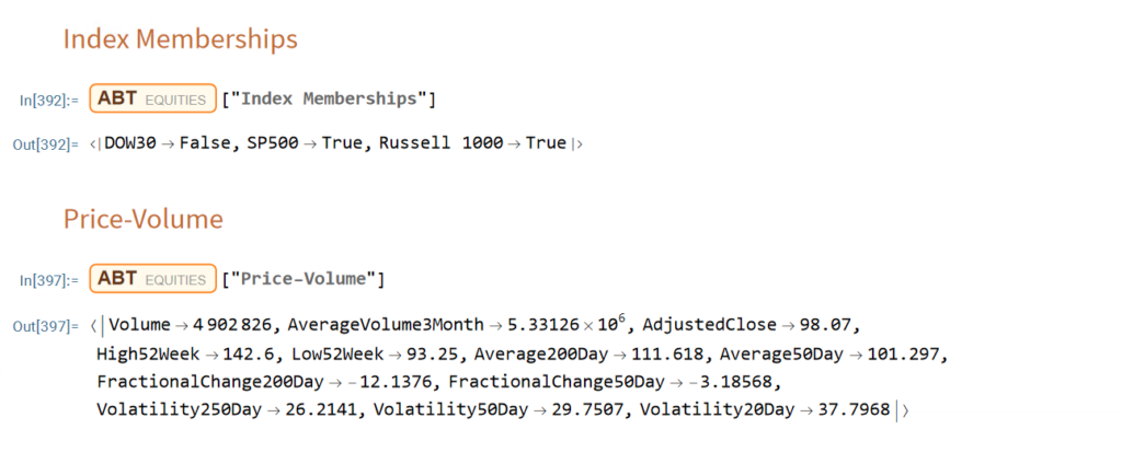
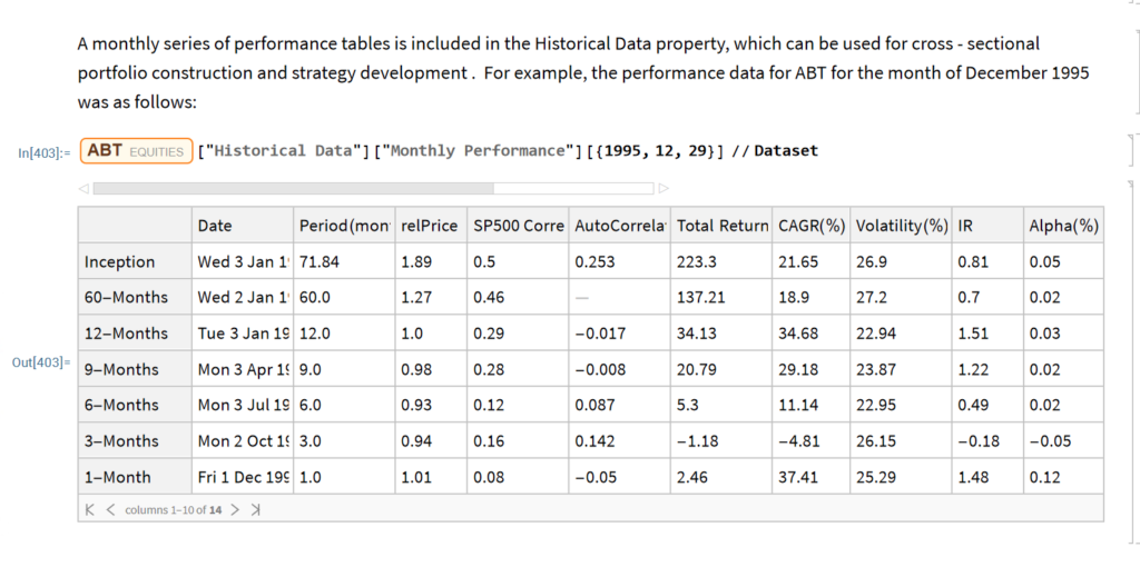
The Equities Entity Store applies the object-oriented concept of Entity Stores in the Wolfram Language to create a collection of equity objects, both stocks and stock indices, containing current and historical fundamental, technical and performance-related data. Also included in the release version of the product will be a collection of utility functions (a.k.a. “Methods”) that will facilitate equity analysis, the formation and evaluation of equity portfolios and the development and back-testing of equities strategies, including cross-sectional strategies.
In the pre-release version of the store there are just over 1,000 equities, but this will rise to over 2,000 in the first release, as delisted securities are added to the store. This is important in order to eliminate survivor bias from the data set.
First Release of the Equities Entity Store – January 2023
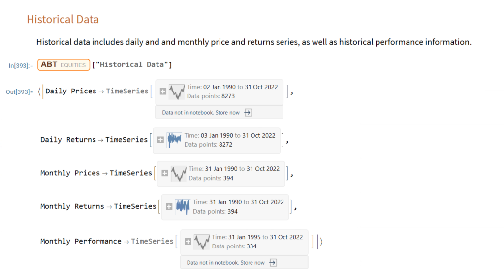
The first release of the equities entity store product will contain around 2,000-2,500 equities, including at least 1,000 active stocks listed on the NYSE and NASDAQ exchanges and a further 1,000-1,500 delisted securities. All of the above information will be available for each equity and, in addition, the historical data will include quarterly fundamental data.
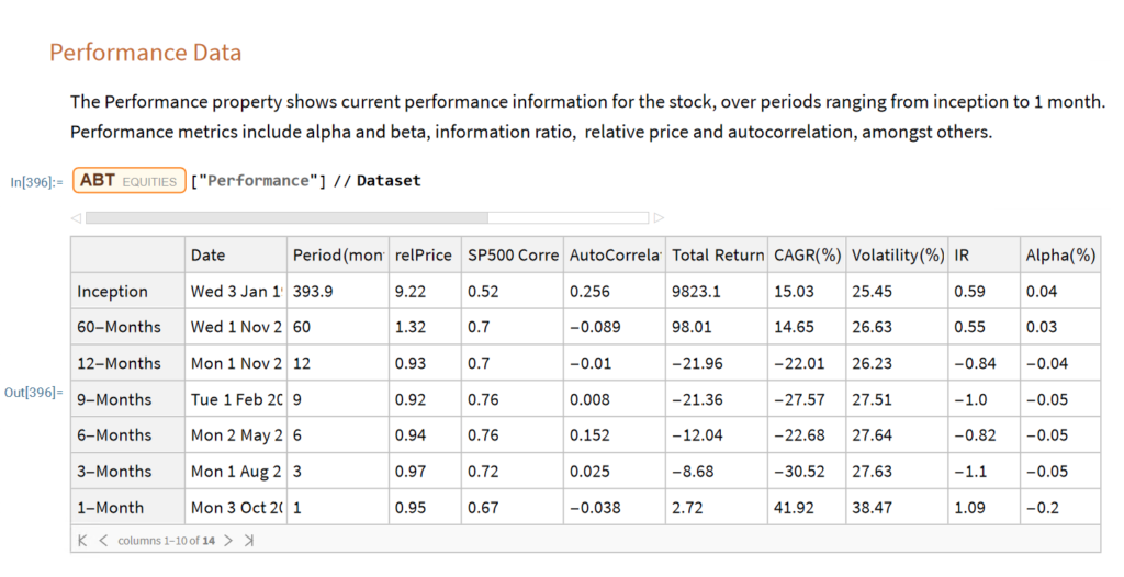
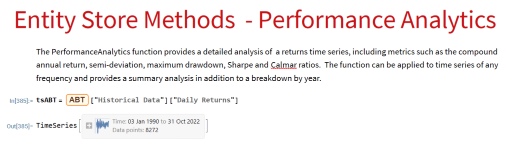
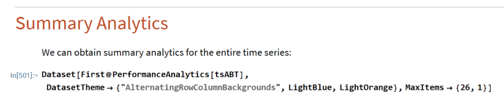
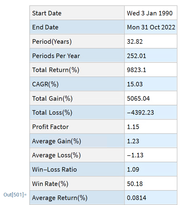
The other major component of the store will be analytics tools, including single-stock analytics functions such as those illustrated here. More important, however, is that the store will contain advanced analytics tools designed to assist the analyst in the construction of optimized equity portfolios and in the development and backtesting of long and long/short equity strategies.
Readers wishing to receive more information should contact me at algosciences (at) gmail.com
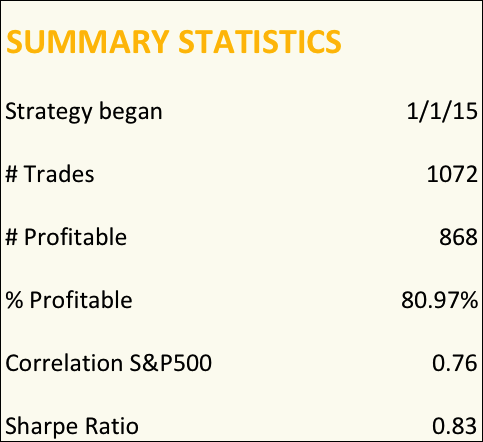
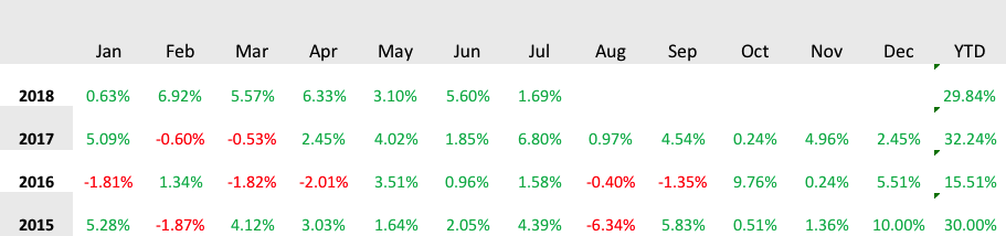
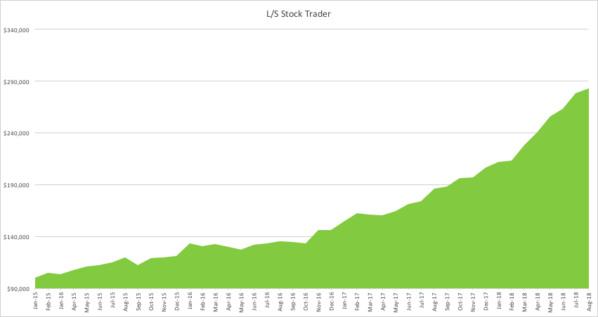
The Long-Short Stock Trader strategy uses a quantitative model to introduce market orders, both entry and exits. The model looks for divergencies between stock price and its current volatility, closing the position when the Price-volatility gap is closed. The strategy is designed to obtain a better return on risk than S&P500 index and the risk management is focused on obtaining a lower drawdown and volatility than index.
The model trades only Large Cap stocks, with high liquidity and without scalability problems. Thanks to the high liquidity, market orders are filled without market impact and at the best market prices.
For more information and back-test results go here.
A few weeks ago I wrote an extensive post on a simple momentum strategy in E-Mini Futures. The basic idea is to buy the S&P500 E-Mini futures when the contract makes a new intraday high. This is subject to the qualification that the Internal Bar Strength fall below a selected threshold level. In order words, after a period of short-term weakness – indicated by the low reading of the Internal Bar Strength – we buy when the futures recover to make a new intraday high, suggesting continued forward momentum.
IBS is quite a useful trading indicator, which you can learn more about in the blog post:
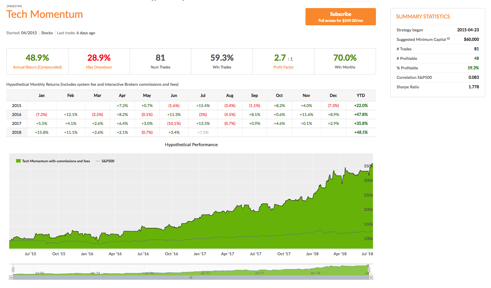
A characteristic of momentum strategies is that they can often be applied successfully across several markets, usually with simple tweaks to the strategy parameters. As a case in point, take our Tech Momentum strategy, listed on the Systematic Strategies Algotrading platform which you can find out more about here:
This swing trading strategy applies similar momentum concepts to exploits long and short momentum effects in technology sector ETFs, focusing on the PROSHARES ULTRAPRO QQQ (TQQQ) and PROSHARES ULTRAPRO SHORT QQQ (SQQQ). Does it work? The results speak for themselves:
In four years of live trading the strategy has produced a compound annual return of 48.9%, with a Sharpe Ratio of 1.78 and Sortino Ratio of 2.98. 2018 is proving to be a banner year for the strategy, which is up by more than 48% YTD.
A very attractive feature of this momentum approach is that it is almost completely uncorrelated with the market and with a beta of just over 1 is hardly more risky than the market portfolio.
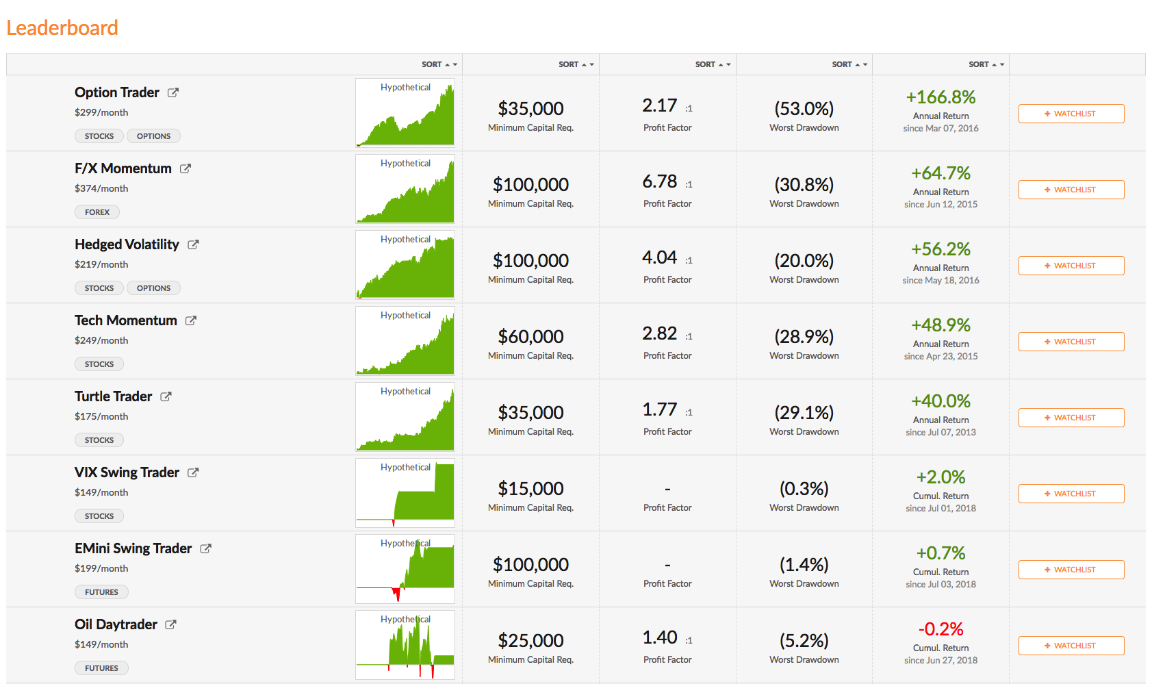
You can find out more about the Tech Momentum and other momentum strategies and how to trade them live in your own account on our Strategy Leaderboard:
Around a quarter of a century ago I wrote a paper entitled “Equity Convexity” which – to my disappointment – was rejected as incomprehensible by the finance professor who reviewed it. But perhaps I should not have expected more: novel theories are rarely well received first time around. I remain convinced the idea has merit and may perhaps revisit it in these pages at some point in future. For now, I would like to discuss a related, but simpler concept: beta convexity. As far as I am aware this, too, is new. At least, while I find it unlikely that it has not already been considered, I am not aware of any reference to it in the literature.
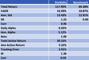
We begin by reviewing the elementary concept of an asset beta, which is the covariance of the return of an asset with the return of the benchmark market index, divided by the variance of the return of the benchmark over a certain period:
Asset betas typically exhibit time dependency and there are numerous methods that can be used to model this feature, including, for instance, the Kalman Filter:
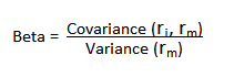
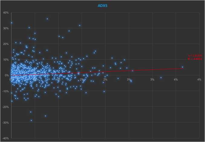
In the context discussed here we set such matters to one side. Instead of considering how an asset beta may vary over time, we look into how it might change depending on the direction of the benchmark index. To take an example, let’s consider the stock Advaxis, Inc. (Nasdaq: ADXS). In the charts below we examine the relationship between the daily stock returns and the returns in the benchmark Russell 3000 Index when the latter are positive and negative.
The charts indicate that the stock beta tends to be higher during down periods in the benchmark index than during periods when the benchmark return is positive. This can happen for two reasons: either the correlation between the asset and the index rises, or the volatility of the asset increases, (or perhaps both) when the overall market declines. In fact, over the period from Jan 2012 to May 2017, the overall stock beta was 1.31, but the up-beta was only 0.44 while the down-beta was 1.53. This is quite a marked difference and regardless of whether the change in beta arises from a change in the correlation or in the stock volatility, it could have a significant impact on the optimal weighting for this stock in an equity portfolio.
Ideally, what we would prefer to see is very little dependence in the relationship between the asset beta and the sign of the underlying benchmark. One way to quantify such dependency is with what I have called Beta Convexity:
Beta Convexity = (Up-Beta – Down-Beta) ^2
A stock with a stable beta, i.e. one for which the difference between the up-beta and down-beta is negligibly small, will have a beta-convexity of zero. One the other hand, a stock that shows instability in its beta relationship with the benchmark will tend to have relatively large beta convexity.
Index Replication using a Minimum Beta-Convexity Portfolio
One way to apply this concept it to use it as a means of stock selection. Regardless of whether a stock’s overall beta is large or small, ideally we want its dependency to be as close to zero as possible, i.e. with near-zero beta-convexity. This is likely to produce greater stability in the composition of the optimal portfolio and eliminate unnecessary and undesirable excess volatility in portfolio returns by reducing nonlinearities in the relationship between the portfolio and benchmark returns.
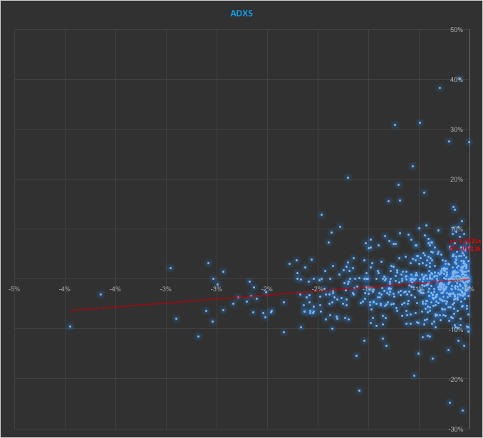
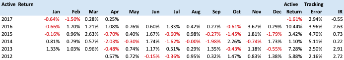
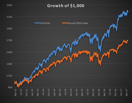
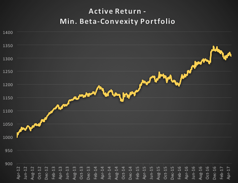
In the following illustration we construct a stock portfolio by choosing the 500 constituents of the benchmark Russell 3000 index that have the lowest beta convexity during the previous 90-day period, rebalancing every quarter (hence all of the results are out-of-sample). The minimum beta-convexity portfolio outperforms the benchmark by a total of 48.6% over the period from Jan 2012-May 2017, with an annual active return of 5.32% and Information Ratio of 1.36. The portfolio tracking error is perhaps rather too large at 3.91%, but perhaps can be further reduced with the inclusion of additional stocks.
Conclusion: Beta Convexity as a New Factor
Beta convexity is a new concept that appears to have a useful role to play in identifying stocks that have stable long term dependency on the benchmark index and constructing index tracking portfolios capable of generating appreciable active returns.
The outperformance of the minimum-convexity portfolio is not the result of a momentum effect, or a systematic bias in the selection of high or low beta stocks. The selection of the 500 lowest beta-convexity stocks in each period is somewhat arbitrary, but illustrates that the approach can scale to a size sufficient to deploy hundreds of millions of dollars of investment capital, or more. A more sensible scheme might be, for example, to select a variable number of stocks based on a predefined tolerance limit on beta-convexity.
Obvious steps from here include experimenting with alternative weighting schemes such as value or beta convexity weighting and further refining the stock selection procedure to reduce the portfolio tracking error.
Further useful applications of the concept are likely to be found in the design of equity long/short and market neural strategies. These I shall leave the reader to explore for now, but I will perhaps return to the topic in a future post.
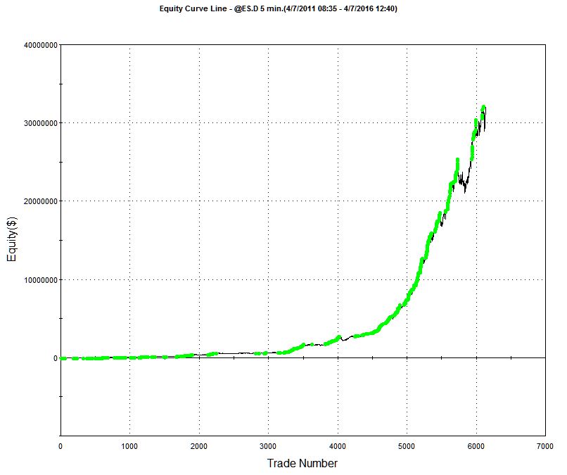
A talented young system developer I know recently reached out to me with an interesting-looking equity curve for a high frequency strategy he had designed in E-mini futures:
Pretty obviously, he had been making creative use of the “money management” techniques so beloved by futures systems designers. I invited him to consider how it would feel to be trading a 1,000-lot E-mini position when the market took a 20 point dive. A $100,000 intra-day drawdown might make the strategy look a little less appealing. On the other hand, if you had already made millions of dollars in the strategy, you might no longer care so much.
A more important criticism of money management techniques is that they are typically highly path-dependent: if you had started your strategy slightly closer to one of the drawdown periods that are almost unnoticeable on the chart, it could have catastrophic consequences for your trading account. The only way to properly evaluate this, I advised, was to backtest the strategy over many hundreds of thousands of test-runs using Monte Carlo simulation. That would reveal all too clearly that the risk of ruin was far larger than might appear from a single backtest.
Next, I asked him whether the strategy was entering and exiting passively, by posting bids and offers, or aggressively, by crossing the spread to sell at the bid and buy at the offer. I had a pretty good idea what his answer would be, given the volume of trades in the strategy and, sure enough he confirmed the strategy was using passive entries and exits. Leaving to one side the challenge of executing a trade for 1,000 contracts in this way, I instead ask him to show me the equity curve for a single contract in the underlying strategy, without the money-management enhancement. It was still very impressive.
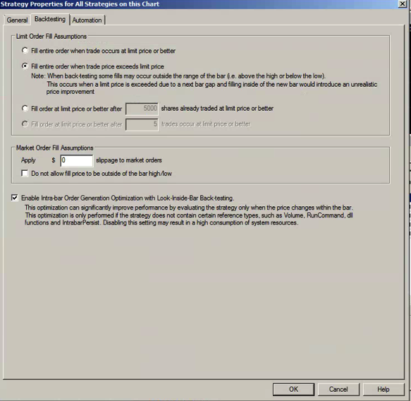
The Critical Fill Assumptions For Passive Strategies
But there is an underlying assumption built into these results, one that I have written about in previous posts: the fill rate. Typically in a retail trading platform like Tradestation the assumption is made that your orders will be filled if a trade occurs at the limit price at which the system is attempting to execute. This default assumption of a 100% fill rate is highly unrealistic. The system’s orders have to compete for priority in the limit order book with the orders of many thousands of other traders, including HFT firms who are likely to beat you to the punch every time. As a consequence, the actual fill rate is likely to be much lower: 10% to 20%, if you are lucky. And many of those fills will be “toxic”: buy orders will be the last to be filled just before the market moves lower and sell orders will be the last to get filled just as the market moves higher. As a result, the actual performance of the strategy will be a very long way from the pretty picture shown in the chart of the hypothetical equity curve.
One way to get a handle on the problem is to make a much more conservative assumption, that your limit orders will only get filled when the market moves through them. This can easily be achieved in a product like Tradestation by selecting the appropriate backtest option:
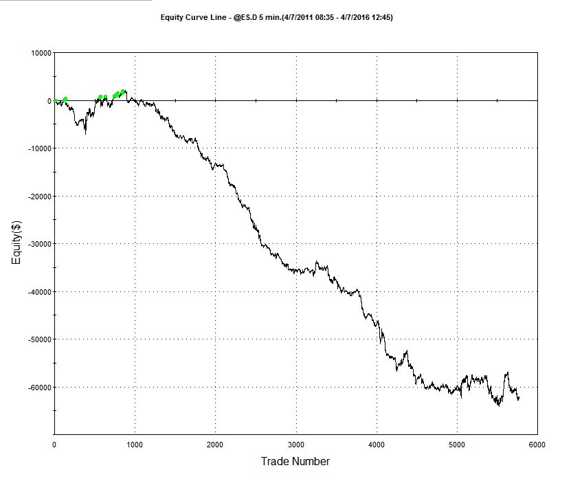
The strategy performance results often look very different when this much more conservative fill assumption is applied. The outcome for this system was not at all unusual:
Of course, the more conservative assumption applied here is also unrealistic: many of the trading system’s sell orders would be filled at the limit price, even if the market failed to move higher (or lower in the case of a buy order). Furthermore, even if they were not filled during the bar-interval in which they were issued, many limit orders posted by the system would be filled in subsequent bars. But the reality is likely to be much closer to the outcome assuming a conservative fill-assumption than an optimistic one. Put another way: if the strategy demonstrates good performance under both pessimistic and optimistic fill assumptions there is a reasonable chance that it will perform well in practice, other considerations aside.
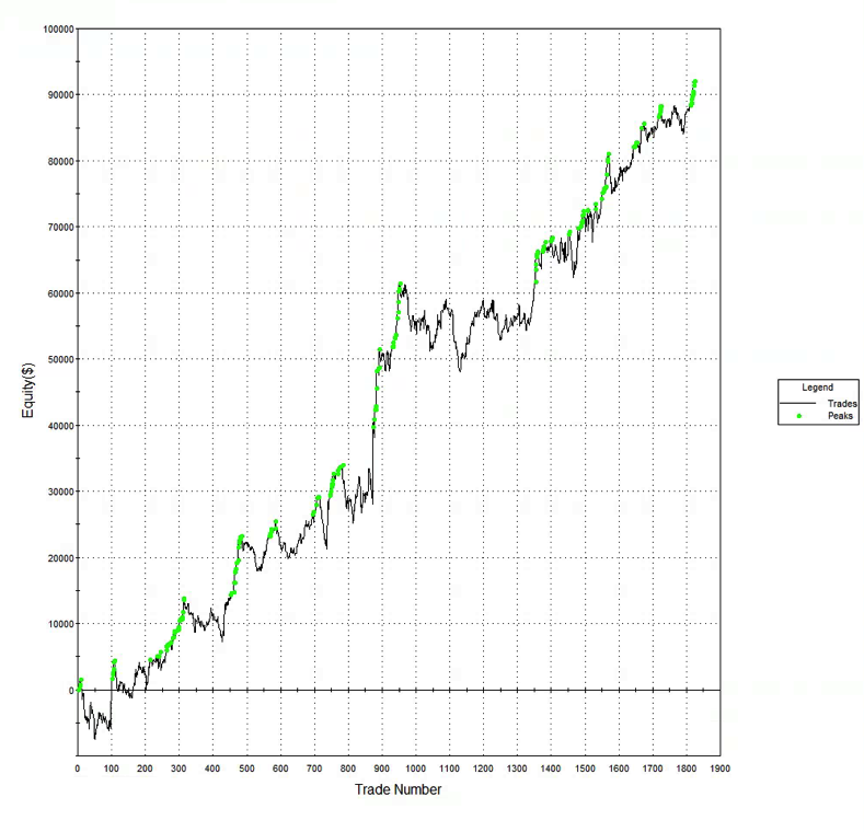
An Example of a HFT Equity Strategy
Let’s contrast the futures strategy with an example of a similar HFT strategy in equities. Under the optimistic fill assumption the equity curve looks as follows:
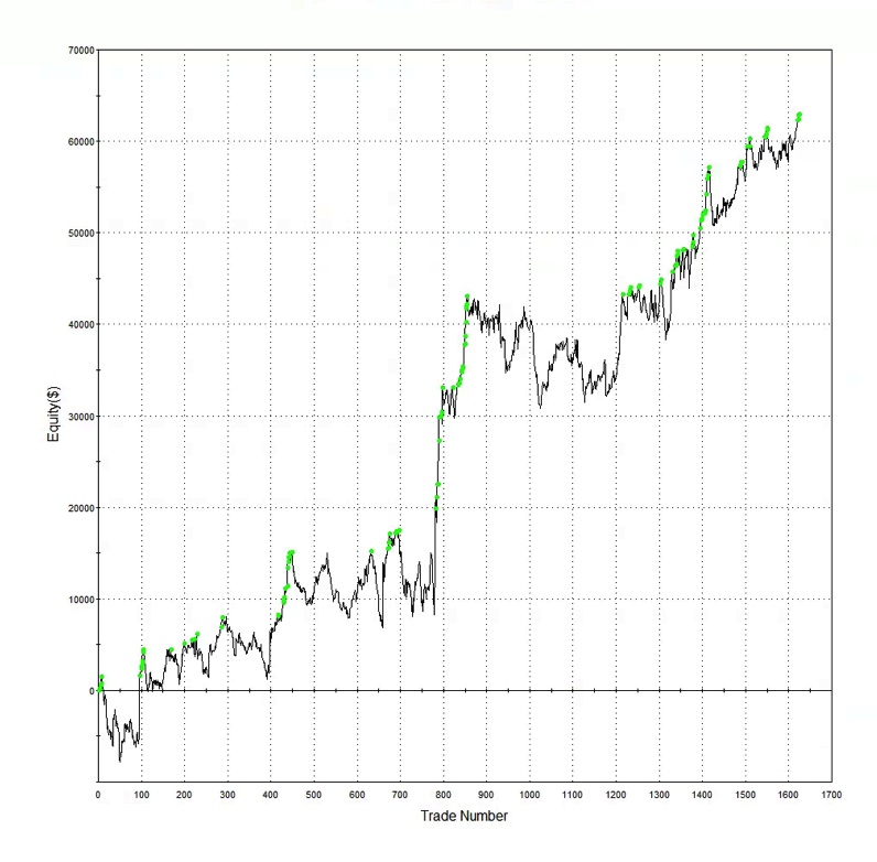
Under the more conservative fill assumption, the equity curve is obviously worse, but the strategy continues to produce excellent returns. In other words, even if the market moves against the system on every single order, trading higher after a sell order is filled, or lower after a buy order is filled, the strategy continues to make money.
Market Microstructure
There is a fundamental reason for the discrepancy in the behavior of the two strategies under different fill scenarios, which relates to the very different microstructure of futures vs. equity markets. In the case of the E-mini strategy the average trade might be, say, $50, which is equivalent to only 4 ticks (each tick is worth $12.50). So the average trade: tick size ratio is around 4:1, at best. In an equity strategy with similar average trade the tick size might be as little as 1 cent. For a futures strategy, crossing the spread to enter or exit a trade more than a handful of times (or missing several limit order entries or exits) will quickly eviscerate the profitability of the system. A HFT system in equities, by contrast, will typically prove more robust, because of the smaller tick size.
Of course, there are many other challenges to high frequency equity trading that futures do not suffer from, such as the multiplicity of trading destinations. This means that, for instance, in a consolidated market data feed your system is likely to see trading opportunities that simply won’t arise in practice due to latency effects in the feed. So the profitability of HFT equity strategies is often overstated, when measured using a consolidated feed. Futures, which are traded on a single exchange, don’t suffer from such difficulties. And there are a host of other differences in the microstructure of futures vs equity markets that the analyst must take account of. But, all that understood, in general I would counsel that equities make an easier starting point for HFT system development, compared to futures.
Commentators have made the point that a high % win rate is not enough.
Yes, you obviously want to pay attention to other performance metrics also, such as profit factor. In fact, there is no reason why you shouldn’t consider an objective function that explicitly combines various desirable performance measures, for example:
net profit * % win rate * profit factor
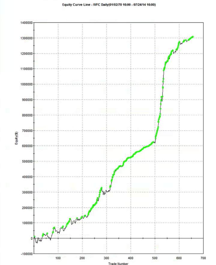
Another approach is to build the model using a data set spanning a different period. I did this with WFC using data from 1990, rather than 1970. Not only was the performance from 1990-2014 better, so too was the performance during the OOS period 1970-1989. Profit factor was 2.49 and %Win rate was 70% across the 44 year period from 1970. For the period from 1990, the performance metrics increase to 3.04 and 73%, respectively.
So in this case, it appears, a most robust strategy resulted from using less data, rather than more. At first this appears counterintuitive. But it’s quite possible for a strategy to be over-condition on behavior that is no longer relevant to the market today. Eliminating such conditioning can sometimes enable strategies to emerge that have greater longevity.