Matlab Archives - QUANTITATIVE RESEARCH AND TRADING

March 4, 2024March 4, 2024

High Frequency Statistical Arbitrage

High-frequency statistical arbitrage leverages sophisticated quantitative models and cutting-edge technology to exploit fleeting inefficiencies in global markets. Pioneered by hedge funds and proprietary trading firms over the last decade, the strategy identifies and capitalizes on sub-second price discrepancies across assets ranging from public equities to foreign exchange.

At its core, statistical arbitrage aims to predict short-term price movements based on probability theory and historical relationships. When implemented at high frequencies—microseconds or milliseconds—the quantitative models uncover trading opportunities unavailable to human traders. The predictive signals are then executable via automated, low-latency infrastructure.

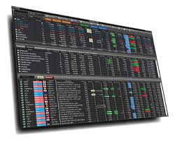
These strategies thrive on speed. By getting pricing data faster, determining anomalies faster, and executing orders faster than the rest of the market, you expand the momentary windows to trade profitably.

Seminal papers have delved into the mathematical and technical nuances underpinning high-frequency statistical arbitrage. Zhaodong Zhong and Jian Wang’s 2014 paper develops stochastic models to quantify how market microstructure and randomness influence high-frequency trading outcomes. Samuel Wong’s 2018 research explores adapting statistical arbitrage for the nascent cryptocurrency markets.

Yet maximizing the strategy’s profitability poses an ongoing challenge. Changing market dynamics necessitate regular algorithm tweaking and infrastructure upgrades. It’s an arms race for lower latency and better predictive signals. Any edge gained disappears quickly as new firms implement similar systems. Regulatory attention also persists due to concerns over unintended impacts on market stability.

Nonetheless, high-frequency statistical arbitrage retains a crucial role for leading quant funds. Ongoing advances in machine learning, cloud computing, and execution technology promise to further empower the strategy. Though the competitive landscape grows more challenging, the cutting edge continues advancing profitably. Where human perception fails, automated high-frequency strategies recognize and seize value.

Implementing an Intraday Statistical Arbitrage Model

While HFT infrastructure and know-how are beyond the reach of most traders, it is possible to conceive of a system for pairs trading at moderate frequency, say 1-minute intervals.

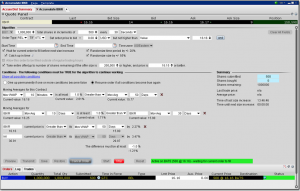
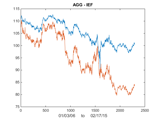
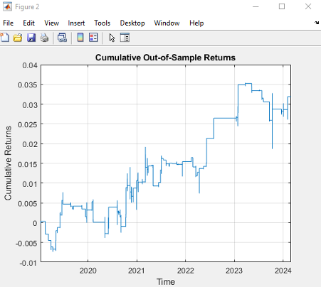
We illustrate the approach with an algorithm that was originally showcased by Mathworks some years ago (but which has since slipped off the radar and is no longer available to download). I’ve amended the code to improve its efficiency, but the core idea remains the same: we conduct a rolling backtest in which data on a pair of assets, in this case spot prices of Brent Crude (LCO) and West Texas Intermediate (WTI), is subdivided into in-sample and out-of-sample periods of varying lengths. We seek to identify windows in which the price series are cointegrated in the sense of Engle-Granger and then apply the regression parameters to take long and short positions in the pair during the corresponding out-of-sample period. The idea is to trade only when there is compelling evidence of cointegration between the two series and to avoid trading at other times.

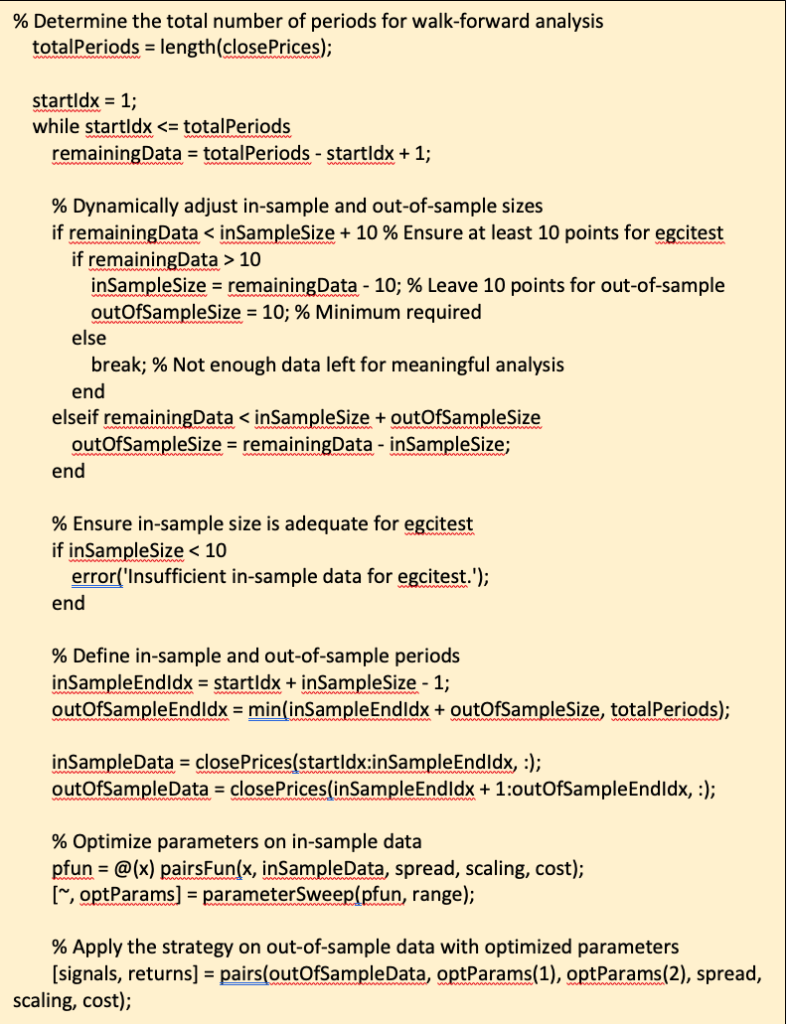
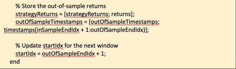
The critical part of the walk-forward analysis code is as shown below. Note we are using a function parametersweep to conduct a grid search across a range of in-sample dataset sizes to determine if the series are cointegrated (according to the Engle-Granger test) in that sub-period and, if so, determine the position size according to the regression parameters. The optimal in-sample parameters are then applied in the out-of-sample period and the performance results are recorded.

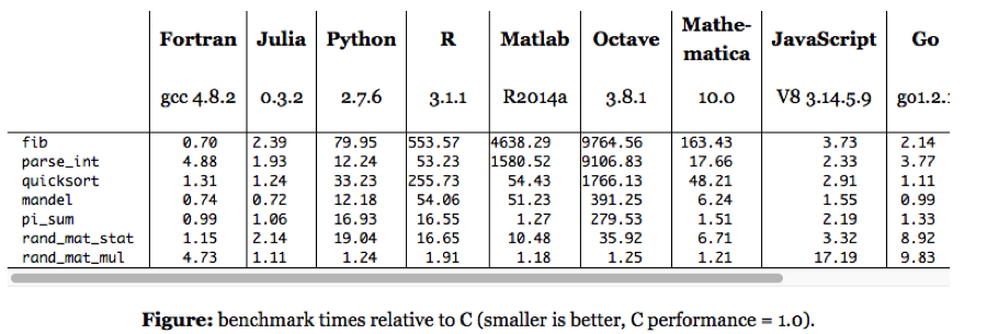
Here we are making use of Matlab’s parallelization capabilities, which work seamlessly to spread the processing load across available CPUs, handling the distribution of variables, function definitions and dependencies with ease. My experience with trying to parallelize Python, by contrast, is often a frustrating one that frequently fails at the first several attempts.

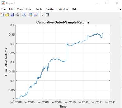
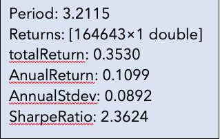
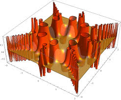
The results appear promising; however, the data is out-of-date, comes from a source that can be less than 100% reliable and may represent price quotes rather than traded prices. If we switch to 1-minute traded prices in a pair of stocks such as PEP and KO that are known to be cointegrated over long horizons, the outcome is very different:

Conclusion

High-frequency statistical arbitrage represents the convergence of cutting-edge technology and quantitative modeling to uncover fleeting trading advantages invisible to human market participants. This strategy has proven profitable for sophisticated hedge funds and prop shops, but also raises broader questions around fairness, regulation, and the future of finance.

However, the competitive edge gained from high-frequency strategies diminishes quickly as the technology diffuses across the industry. Firms must run faster just to stand still.

Continued advancement in machine learning, cloud computing, and execution infrastructure promises to expand the frontier. But practitioners and policymakers alike share responsibility for ensuring market integrity and stability amidst this technology arms race.

In conclusion, high-frequency statistical arbitrage remains essential to many leading quantitative firms, with the competitive landscape growing ever more challenging. Realizing the potential of emerging innovations, while promoting healthy markets that benefit all participants, will require both vision and wisdom. The path ahead lies between cooperation and competition, ethics and incentives. By bridging these domains, high-frequency strategies can contribute positively to financial evolution while capturing sustainable edge.

References:

Zhong, Zhaodong, and Jian Wang. “High-Frequency Trading and Probability Theory.” (2014).

Wong, Samuel S. Y. “A High-Frequency Algorithmic Trading Strategy for Cryptocurrency.” (2018).

Glossary

For those unfamiliar with the topic of statistical arbitrage and its commonly used terms and concepts, check out my book Equity Analytics, which covers the subject matter in considerable detail.

March 1, 2024March 4, 2024

Matlab vs. Python

In a previous article I made a detailed comparison of Mathematica and Python and tried to identify areas where the former excels. Despite the many advantages of the Python technology stack, I was able to pinpoint a few areas in which I think Mathematica holds the upper hand. Whether those are sufficient to warrant the investment of time and money required to master the Wolfram Language is another matter, which the user must decide for himself.

In this comparison between Matlab and Python I won’t reiterate the strengths of the Python that make it the programming language of choice for so many developers. Let me instead focus on some of the key aspects of Matlab where I think the Mathworks product outshines its rival.

Matlab is designed for numerical computing, while Python is a general-purpose programming language that has become a major tool for scientific computing through libraries like NumPy, SciPy, and Matplotlib.

The key advantages of Matlab relative to Python, as I see them, are as follows:

Integrated Development Environment (IDE):

Matlab comes with a feature-rich IDE that is tailored for mathematical and engineering workflows. This includes tools for debugging, data visualization, GUI creation, and managing workspace variables. The Matlab IDE is specifically designed to streamline the development of mathematical and engineering applications.

Advanced Toolboxes:

Matlab offers a wide range of specialized toolboxes for different applications, including signal processing, control systems, neural networks, image processing, and many others. These toolboxes are professionally developed, rigorously tested, and regularly updated, providing a comprehensive suite of algorithms and functions for specific domains. With its vast ecosystem of scientific libraries Python has caught up with Matlab in recent years, and even overtaken it in some areas, but Matlab’s toolboxes are tried and battle-tested technologies that are used by millions of users in state-of-the-art applications.

Simulink:

Matlab provides Simulink, a platform for Model-Based Design for dynamic and embedded systems. Simulink is a graphical programming environment for modeling, simulating, and analyzing multidomain dynamical systems. This is particularly useful in engineering applications where system modeling and simulation are crucial.

Built-in Support for Matrix Operations:

Matlab (Matrix Laboratory) has inherent support for matrix operations and linear algebra, making it highly efficient for tasks that involve complex mathematical computations.

Performance:

Matlab is optimized for operations involving matrices and vectors, which are central to engineering and scientific computations. For certain numerical tasks, Matlab’s performance is superior due to its highly optimized code and ability to handle parallel computing and GPU acceleration effectively.

Matlab’s speed has further accelerated over the last decade due to just-in-time compilation. This feature automatically compiles Matlab’s interpreted code into machine code at runtime, which speeds up execution, especially in loops and computationally intensive tasks. The JIT compilation process is entirely transparent to the user, requiring no modifications to the code or the development process.
Python itself is an interpreted language and does not include JIT compilation in its standard implementation (CPython). However, JIT compilation can be introduced through third-party libraries or alternative Python implementations, such as Numba or PyPy.

Testing and Debugging:

Both Matlab and Python are equipped with robust testing and debugging tools that cater to their specific user bases. Matlab’s tools are tightly integrated into its IDE and are particularly tailored for numerical computing and engineering tasks. I would regard them as the industry standard in terms of features, ease of use and helpfulness. In contrast, Python’s testing and debugging ecosystem is more diverse, with multiple options available for different tasks, including third-party libraries that extend its capabilities.

Documentation and Support:

Matlab’s documentation is extensive, well-organized, and includes examples for a wide range of functions and toolboxes. Additionally, MathWorks provides excellent support services, including technical support and community forums, which can be particularly valuable for complex or specialized projects.

Conclusion

While Python has gained significant popularity in scientific computing, data science, and machine learning due to its open-source nature and the vast ecosystem of libraries, Matlab holds strong advantages in numerical computing, engineering applications, and when integrated solutions with robust support and documentation are required.

However, Python offers greater flexibility, scalability and has grown significantly in scientific computing. MATLAB historically had limitations with very large datasets, but recent releases have added features to improve performance with big data. Still, Python likely retains an advantage for extreme scales. The choice depends on the specific use case – for small-scale numerical computing and modeling MATLAB provides an integrated optimized environment while Python excels in general-purpose programming and very large-scale data intensive applications. However, both continue to evolve impressive capabilities so the lines are blurring. Ultimately data scientists and engineers are best served by being proficient in both languages.

October 16, 2018

Algorithmic Trading

MOVING FROM RESEARCH TO TRADING

I have written recently about the comparative advantages of different programming languages in the context of research and trading (see here). My sense of it is that there is no single “ideal” programming language – the best strategy is to pick an appropriate tool for the job and there are usually several reasonable choices one could make.

If you are engaged in econometrics research, you might choose a package like RATS, Eviews, Gauss, or Prof. James Davidson’s excellent and inexpensive TSM, which I have used for many years and can recommend highly. For a latency-sensitive high frequency trading application, you will probably want to use something like C++, or possibly a 3rd party algo system like Apama or Tethys. But for algorithmic trading systems of intermediate frequency the choice appears almost unlimited.

The problem with retail trading tools like TradeStation, Multicharts, or Amibroker, is that they are designed primarily for single-asset strategies. That may be ok for futures trading,where more often than not the focus is on a single underlying, but in equities the opposite is true. Using one of these products to develop and implement a pairs trading strategy is a stretch. As for portfolio analytics – forget it.

This is where more general, high level languages like R, Matlab or Mathematica come in: their greater power and flexibility is handling large, multivariate data sets makes it much more straightforward to develop portfolio strategies. And they can often bridge the gap between R&D and implementation quite easily: code that was used in the research stage can often be quickly re-tooled to work in a production version of the system. As for production systems, there is now a significant cottage industry of traders who use Matlab in algo trading. R has a similar following (see here).

In addition to parallelizing the code (for use with the Parallel Computing Toolbox) to speed up the research phase, you might also want to implement a hybrid system by re-coding the slower routines in C++, to create a mex file (for details see here). Matlab’s Profiler is a useful tool for identifying code bottlenecks. In a recent piece of research in which I was evaluating over 30,000,000 cointegrated portfolios, I discovered to my surprise that the main code bottleneck was the multiple calls to Matlab’s std function, a problem easily fixed with a few lines of C++ code. The resulting hybrid program executed at more than twice the speed – important when your run time might be several hours, or even days.

HOOKING UP THE EXECUTION PLATFORM

The main challenge for developers using generic tools like Mathematica, Matlab or R is the implementation stage of the project. Providing connectivity to brokerage/execution platforms never seemed high on the list of priorities for Wolfram or Mathworks and things are similarly hit or miss with R.

Belatedly, Mathematica now offers a link to Bloomberg via its Finance Platform. Matlab, meanwhile, offers a Trading Toolbox, which supposedly offers connectivity , not only to Bloomberg, but also Interactive Brokers and Trading Technologies, amongst other platforms. Unfortunately, the toolbox interface to IB appears to rely on outdated 1990s ActiveX technology, which is flakey at best. In tests, I was unable to make progress past the ‘not connected’ error message.

At that point I turned to Yair Altman’s IB-Matlab product. Happily, this uses IB’s Java api, which is a great deal more robust than the ActiveX platform. It’s been some time since I last used IB-Matlab and was pleased to see that Yair has been very busy over the intervening period, building the capabilities of the system and providing very comprehensive documentation for it. With Yair’s help, it took me no time at all to get up and running and within a day or two the system was executing orders flawlessly in IB’s TWS. The relatively few snags I ran into were almost all due to IB’s extremely terse error messaging, which often gives almost no clue as to what the issue might be. Fortunately, Yair is very generous with his time in providing support to his users and his responses to me questions were fast and detailed.

EXECUTION ALGOS

With intermediate systems trading at frequencies of, say, 5-minutes to daily, one has a choice to make as regards execution. Given that the strategy is not very latency sensitive, it is certainly conceivable to develop one’s own execution algos in Matlab. However, platforms like TWS are equipped with native algos, not only from IB, but also other providers like Credit Suisse and Jeffries.

Actually, I have found several of IB’s own algos such as Scaletrader and Accumulate/Distribute to be very effective. Certainly IB seems very proud of them – IB CEO Thomas Peterffy has patented at least one of them. Accumulate/Distribute, for instance, is quite sophisticated, allowing the user to randomize and slice the size and interval between individual orders, use passive or aggressive order types, and pause execution on a news alert, or when the price falls below a moving average, or outside a specified range.

There is much to be said for using algos native to the execution platform rather than reinventing the wheel, providing the cost is reasonable. So, while it is perfectly feasible to build execution algos in Matlab, it typically isn’t necessary – in most cases standard algos will suffice.

There are exceptions, of course. IB doesn’t offer the kind of basket-trading capabilities that are available in advanced algo platforms like Tethys or RediPlus. In those systems, for example, you can set the level of long/short imbalance in the portfolio that you are willing to tolerate and the algo will speed up or slow down execution of trades in individual components of the basket to maintain the dollar imbalance within that tolerance. You can also manage the sector risk dynamically during execution.

Those kind of advanced capabilities don’t come cheap and you wont find them at IB, or any other retail platform. If you need that kind of functionality, for example, because you are trading a long/short equity portfolio within a universe of 200-300 names, your best option is probably to switch to a different execution platform. Otherwise you will need to code a custom algo in your language of choice.

For many quantitative strategies, (at least the low frequency ones) IB’s standard algos are often good enough. The Accumulate/Distribute algo, for instance, will show a visual representation of the progress of the execution of individuals legs of a pairs trade, and it is easy enough to identify a potential imbalance and adjust the algo parameters in real time. If you are only trading pairs, or small portfolios of cointegrated securities, it probably isn’t worthwhile to develop the sophisticated logic that would be required to handle the adjustment of the execution of individual legs of a trade in a fully automated way. A large portfolio would be a different matter, however.

MATLAB EXAMPLE

I thought it might be instructive to take a look at how you might implement the execution of a strategy in Matlab, using IB algos. In the Matlab code fragment below, the (2 x nTickers) array tradeActions contains, in the first row, the action we wish to take (1 = BUY, -1 = SELL, -2 = SELL SHORT) and in the second row the (absolute value of) the number of shares we wish to trade for tickers i =1:nTickers. We break each order up into hundred lots and odd lots, routing the former via IB’s Accumulate/Distribute algo and the latter as passive REL orders (note that A/D will typically randomize the timing of each sub-order, while REL orders are posted directly into the market). The Matlab function AccumulateDistribute implements the most important features of IB’s A/D algo, including random size and time slicing of the order. Orders are submitted as passive REL orders with zero offset (so they will sit on the current bid or ask) – obviously you would typically want to consider allowing some non-zero offset for less liquid securities. It is not hard to envisage how one might further enhance the algo to monitor the progress of the execution and speed up or slow down certain orders accordingly.

A couple of IB api “gotchas” to be aware of:

(i) IB requires unique and monotonically increasing orderIds for each order. One way to do this, suggested by Yair, is to use orderId = round((now-735000)*3e5); This fails when you are submitting a number of orders sequentially at high speed (say in a for loop), where the time increments are sub-second, so you need to pass the orderID back and force a minimal increment, as I have in the code below.

(ii) It is very important to specify the primary exchange of each security: securities with identical tickers can be found trading on different exchanges. Failing to specify the primary exchange in such a case will result in IB rejecting the order with a typically cryptic api message.

Continue reading “Algorithmic Trading”

October 2, 2018

A Comparison of Programming Languages

Towards the end of last year I wrote a post (see here) about the advent of modern programming languages, including the JIT compiled Julia and visual programming language ADL from Trading Technologies. My conclusion (based on a not very scientific sample) was that we appear to be at the tipping point, where the speed of newer, high level languages languages is approaching that of the fastest compiled languages like C/C++.

Now comes a formal academic study of the topic in A Comparison of Programming Languages in Economics, Aruoba and Fernandez-Villaverde, 2014. Using the neoclassical growth model, the authors conduct a benchmark test in C++11, Fortran 2008, Java, Julia, Python, Matlab, Mathematica, and R, implementing the same algorithm, value function
iteration with grid search, in each of the languages. They report the execution times of the codes in a Mac and in a Windows computer and briefly comment on the strengths and weaknesses of each language.

The conclusions from the study mirror my own thoughts on the subject very closely. The authors find that:

C++ and Fortran are still considerably faster than any other alternative, although one needs to be careful with the choice of compiler.
C++ compilers have advanced enough that, contrary to the situation in the 1990s and some folk wisdom, C++ code runs slightly faster (5-7 percent) than Fortran code.
Julia delivers outstanding performance. Execution speed is only between 2.64 and 2.70 times slower than the execution speed of the best C++ compiler.
Baseline Python was slow. Using the Pypy implementation, it runs around 44 times slower than in C++. Using the default CPython interpreter, the code runs between 155 and 269 times slower than in C++.
Matlab is between 9 to 11 times slower than the best C++ executable.
R runs between 475 to 491 times slower than C++. If the code is compiled, the code is between 243 to 282 times slower.
Hybrid programming and special approaches can deliver considerable speed ups. For example, when combined with Mex files, Matlab is only 1.24 to 1.64 times slower than C++ and when combined with Rcpp, R is between 3.66 and 5.41 times slower. Similar numbers hold for Numba (a just-in-time compiler for Python that uses decorators) and Cython (a static compiler for writing C extensions for Python) in the Python ecosystem.
Mathematica is only about three times slower than C++, but only after a considerable rewriting of the code to take advantage of the peculiarities of the language. The baseline version of the algorithm in Mathematica is considerably slower.

C++ still represents the benchmark for speed, but not by much. It is barely faster than the old stalwart, Fortran, and only 1.5 – 3 times faster than up-and-coming rivals amongst the higher level languages (especially when you allow for hybrid programming to speed up the slowest algorithms).

So, as regards developing financial models and trading systems, my questions are (as before):

Why would anyone prefer Python, given that there is a much faster, free alternative in Julia, which is just as easy a language to program in?
What justification is there for preferring R to Matlab, other than cost?
Why does anyone bother with Java? If speed is the critical issue, there are faster alternatives. If you like the relative simplicity of the syntax, Julia is cleaner, simpler and just as fast in execution.

When you reach a point where a high level language like Matlab is only around 1.5x – 2x slower than C++, you really have to question whether the latter is an appropriate choice. Yes, of course, in mission-critical applications where you need access to the hardware layer for speed purposes, C++ is the way to go. But for so many applications, that just isn’t the case.

What matters, far, far more, are the months of costly and laborious programming effort that is often required to reproduce basic functionality that is already embedded in higher level languages like Matlab or Mathematica. Not only that, but the end result of a C++ /Java development effort is likely to be notoriously inflexible by comparison. That’s a huge drawback. Rarely, if ever, does a piece of research translate flawlessly into production – it requires one to iterate towards a final solution, often making significant changes to the design of the system in the light of practical experience.

If I had to guess, based on my experience, I would say that 80% or more of development tasks in quantitative research and trading would produce a superior result if preference was given to using a higher level language for the initial development. When the system is sufficiently stable to put into production, you simply create a hybrid application by recoding any mission-critical components for which speed is an issue in C++.

Finally, where does that leave my beloved Mathematica? To be fair, while you don’t have the joys of strong typing to contend with, Mathematica’s syntax is just as demanding and uncompromising as C++ – a missed comma or incorrectly placed bracket is just as critical. But, the point is, while in C++ the syntactical rigor is just annoying, in Mathematica it’s worth putting up with because the productivity is so much greater. A competent programmer can produce, in a single line of Mathematica code, a program that would require hundreds, if not thousands of lines of C++ code to accomplish. Sure, he might get the syntax wrong at first: but it’s only a single line of code and the interactive gui interface makes debugging very simple.

That said, while Mathematica can be very tedious to use for procedural programming, it excels in three areas:

1. Symbolic programming. Anything involving mathematical symbols and equations – Mathematica is #1

2. User interface. In Mathematica, it is trivial to build a sophisticated, dynamic gui in no time at all, again, often in 1-2 lines of code

3. Functional programming. Anything that can be thought of as a function, Mathematica handles extremely well. We are not talking about finding a square root here: I mean extremely complex functions that, again, might take hundreds of lines of code in another language.

It is also worth pointing out that Mathematica comes supplied with functionality that Matlab provides only through numerous, costly add-on packages.

CONCLUSION
Before I allow a development team to start mindlessly coding up a system in Java or C++, I want to hear their reasons why they aren’t going to do it 10x faster in another, higher level language. “We always use C++/Java for production” is not a reason. Specifically, which parts of the system require the additional 1.5x speed-up, and why can’t they be coded as dlls (Matlab mex functions)?

Finally, on a cost-benefit basis, ask yourself how much you might benefit if the months and tens (or hundreds) of thousands of dollars wasted on developing in C++ were instead spent on researching and developing new trading ideas.

October 1, 2018

ETF Pairs Trading with the Kalman Filter

I was asked by a reader if I could illustrate the application of the Kalman Filter technique described in my previous post with an example. Let’s take the ETF pair AGG IEF, using daily data from Jan 2006 to Feb 2015 to estimate the model. As you can see from the chart in Fig. 1, the pair have been highly correlated over the last several years.

Fig 1. AGG and IEF Daily Prices 2006-2015

We now estimate the beta-relationship between the ETF pair with the Kalman Filter, using the Matlab code given below, and plot the estimated vs actual prices of the first ETF, AGG in Fig 2. There are one or two outliers that you might want to take a look at, but mostly the fit looks very good.

Fig 2 – Actual vs Fitted Prices of AGG

Now lets take a look at Kalman Filter estimates of beta. As you can see in Fig 3, it wanders around a lot! Very difficult to handle using some kind of static beta estimate.

Fig 3 – Kalman Filter Beta Estimates

Finally, we compute the raw and standardized alphas, being the differences between the observed and fitted prices , i.e. Alpha(t) = AGG(t) – b(t)* IEF(t) and kfAlpha(t) = (Alpha(t) – mean(Alpha(t)) / std(Alpha(t) I have plotted the kfAlpha estimates over the last year in Fig 4.

Fig 4 – Standardized Alpha Estimates

The last step is to decide how to trade this relationship. You might, for example, trade the portfolio in proportion to the standardized deviation (i.e. the size of kfAlpha(t)). Alternatively, you might set a threshold level, say +/- 1 Sd, and trade the portfolio when kfAlpha(t) exceeds this the threshold. In the Matlab code below I use the particle swarm method to maximize the likelihood. I have found this to be more reliable than other methods.

Continue reading “ETF Pairs Trading with the Kalman Filter”

September 25, 2018

Just in Time: Programming Grows Up – JonathanKinlay.com

Move over C++: Modern Programming Languages Combine Productivity and Efficiency

Like many in the field of quantitative research, I have programmed in several different languages over the years: Assembler, Fortran, Algol, Pascal, APL, VB, C, C++, C#, Matlab, R, Mathematica. There is an even longer list of languages I have never bothered with: Cobol, Java, Python, to name but three.

In general, the differences between many of these are much fewer than their similarities: they reserve memory; they have operators; they loop. Several have ghastly syntax requiring random punctuation that supposedly makes the code more intelligible, but in practice does precisely the opposite. Some, like Objective C, are so ugly and poorly designed they should have been strangled at birth. The ubiquity of C is due, not to its elegance, but to the fact that it was one of the first languages distributed for free to impecunious students. The greatest benefit of most languages is that they compile to machine code that executes quickly. But the task of coding in them is often an unpleasant, inefficient process that typically involves reinvention of the wheel multiple times over and massive amounts of tedious debugging. Who, after all, doesn’t enjoy unintelligible error messages like “parsec error in dynamic memory heap allocator” – when the alternative, comprehensible version would be so prosaic: “in line 51 you missed one of those curly brackets we insist on for no good reason”.

There have been relatively few steps forward that actually have had any real significance. Most times, the software industry operates rather like the motor industry: while the consumer pines for, say, a new kind of motor that will do 1,000 miles to the gallon without looking like an electric golf cart, manufacturers announce, to enormous fanfare, trivia like heated wing mirrors.

The first language I came across that seemed like a material advance was APL, a matrix-based language that offers lots of built-in functionality, very much like MatLab. Achieving useful end-results in a matter of days or weeks, rather than months, remains one of the great benefits of such high-level languages. Unfortunately, like all high-level languages that are weakly typed, APL, MatLab, R, etc, are interpreted rather than compiled. And so I learned about the perennial trade-off that has plagued systems development over the last 30 years: programming productivity vs. execution efficiency. The great divide between high level, interpreted languages and lower-level, compiled languages, would remain forever, programming language experts assured us, because of the lack of type-specificity in the former.

High-level language designers did what they could, offering ever-larger collections of sophisticated, built-in operators and libraries that use efficient machine-code instructions, as well as features such as parallel processing, to speed up execution. But, while it is now feasible to develop smaller applications in a few lines of Matlab or Mathematica that have perfectly acceptable performance characteristics, major applications (trading platforms, for example) seemed ordained to languish forever in the province of languages whose chief characteristic appears to be the lack of intelligibility of their syntax.

I was always suspicious of this thesis. It seemed to me that it should not be beyond the wit of man to design a programming language that offers straightforward, type-agnostic syntax that can be compiled. And lo: this now appears to have come true.

Of the multitude of examples that will no doubt be offered up over the next several years I want to mention two – not because I believe them to be the “final word” on this important topic, but simply as exemplars of what is now possible, as well as harbingers of what is to come.

Trading Technologies ADL

The first, Trading Technologies’ ADL, I have written about at length already. In essence, ADL is a visual programming language focused on trading system development. ADL allows the programmer to deploy highly-efficient, pre-built code blocks as icons that are dragged and dropped onto a programming canvass and assembled together using logic connections represented by lines drawn on the canvass. From my experience, ADL outpaces any other high-level development tool by at least an order of magnitude, but without sacrificing (much) efficiency in execution, firstly because the code blocks are written in native C#, and secondly, because completed systems are deployed on an algo server with a sub-millisecond connectivity to the exchange.

The second example is a language called Julia, which you can find out more about here. To quote from the web site:

“Julia is a high-level, high-performance dynamic programming language for technical computing. Julia features optional typing, multiple dispatch, and good performance, achieved using type inference and just-in-time (JIT) compilation, implemented using LLVM”

The language syntax is indeed very straightforward and logical. As to performance, the evidence appears to be that it is possible to achieve execution speeds that match or even exceed those achieved by languages like Java or C++.

How High Level Programming Languages Match Up

The following micro-benchmark results, provided on the Julia web site, were obtained on a single core (serial execution) on an Intel® Xeon® CPU E7-8850 2.00GHz CPU with 1TB of 1067MHz DDR3 RAM, running Linux:

We need not pretend that this represents any kind of comprehensive speed test of Julia or its competitors. Still, it’s worth dwelling on a few of the salient results. The first thing that strikes me is how efficient Fortran, the grand-daddy of programming languages, remains in comparison to more modern alternatives, including the C benchmark. The second result I find striking is how slow the much-touted Python is compared to Julia, Go and C. The third result is how poorly MatLab, Octave and R perform on several of the tests. Finally, and in some ways the greatest surprise at all is the execution efficiency of Mathematica relative to other high-level languages like MatLab and R. It appears that Wolfram has made enormous progress in improving the speed of Mathematica, presumably through the vast expansion of highly efficient built-in operators and functions that have been added in recent releases (see chart below).

Source: Wolfram

Mathematica even compares favorably to Python on several of the tests. Given that, why would anyone spend time learning a language like Python, which offers neither the development advantages of Mathematica, nor the speed advantages of C (or Fortran, Java or Julia)?

In any event, the main point is this: it appears that, in 2015, we can finally look forward to dispensing with legacy programing languages and their primitive syntax and instead develop large, scalable systems that combine programming productivity and execution efficiency. And that is reason enough for any self-respecting quant to rejoice.

My best wishes to you all for the New Year.