VIX Index Archives - QUANTITATIVE RESEARCH AND TRADING

July 28, 2020

Volatility Trading Styles

The VIX Surge of Feb 2018

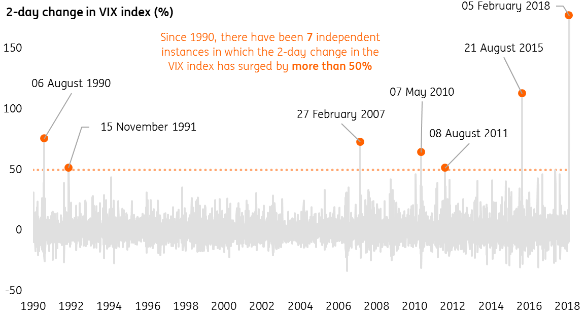
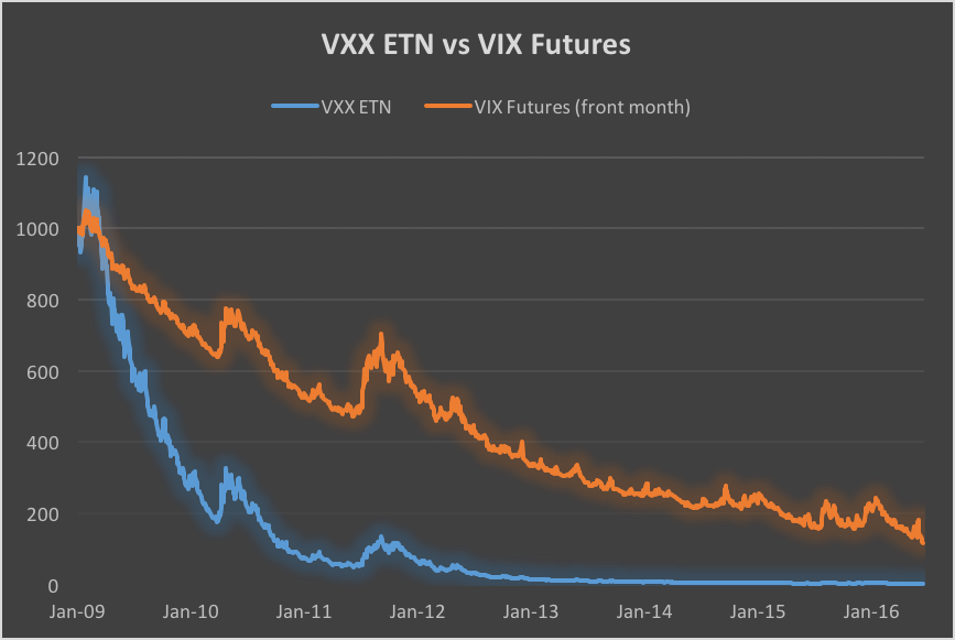
Volatility trading has become a popular niche in investing circles over the last several years. It is easy to understand why: with yields at record lows it has been challenging to find an alternative to equities that offers a respectable return. Volatility, however, continues to be volatile (which is a good thing in this context) and the steepness of the volatility curve has offered investors attractive returns by means of the volatility carry trade. In this type of volatility trading the long end of the vol curve is sold, often using longer dated futures in the CBOE VIX Index, for example. The idea is that profits are generated as the contract moves towards expiration, “riding down” the volatility curve as it does so. This is a variant of the ever-popular “riding down the yield curve” strategy, a staple of fixed income traders for many decades. The only question here is what to use to hedge the short volatility exposure – highly correlated S&P500 futures are a popular choice, but the resulting portfolio is exposed to significant basis risk. Besides, when the volatility curve flatten and inverts, as it did in spectacular fashion in February, the transition tends to happen very quickly, producing a substantial losses on the portfolio. These may be temporary, if the volatility spike is small or short-lived, but as traders and investors discovered in the February drama, neither of these two desirable outcomes is guaranteed. Indeed as I pointed out in an earlier post this turned out to be the largest ever two-day volatility surge in history. The results for many hedge funds, especially in the quant sector were devastating, with several showing high single digit or double-digit losses for the month.

Over time, investors have become more familiar with the volatility space and have learned to be wary of strategies like volatility carry or option selling, where the returns look superficially attractive, until a market event occurs. So what alternative approaches are available?

An Aggressive Approach to Volatility Trading

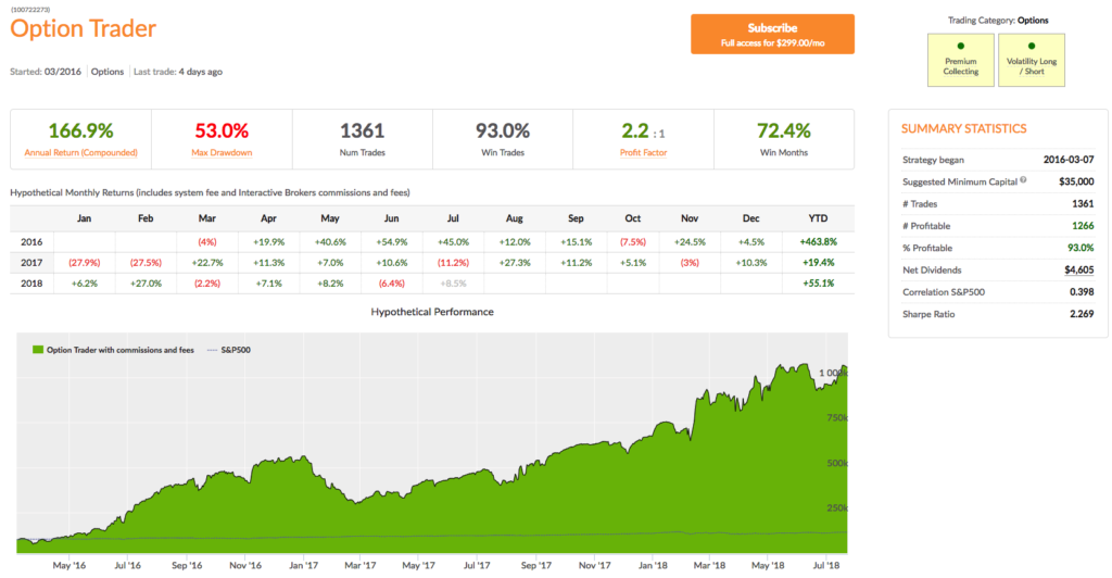
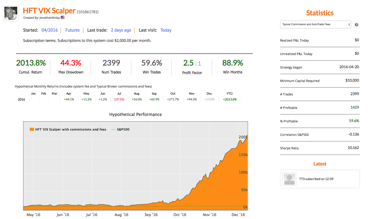
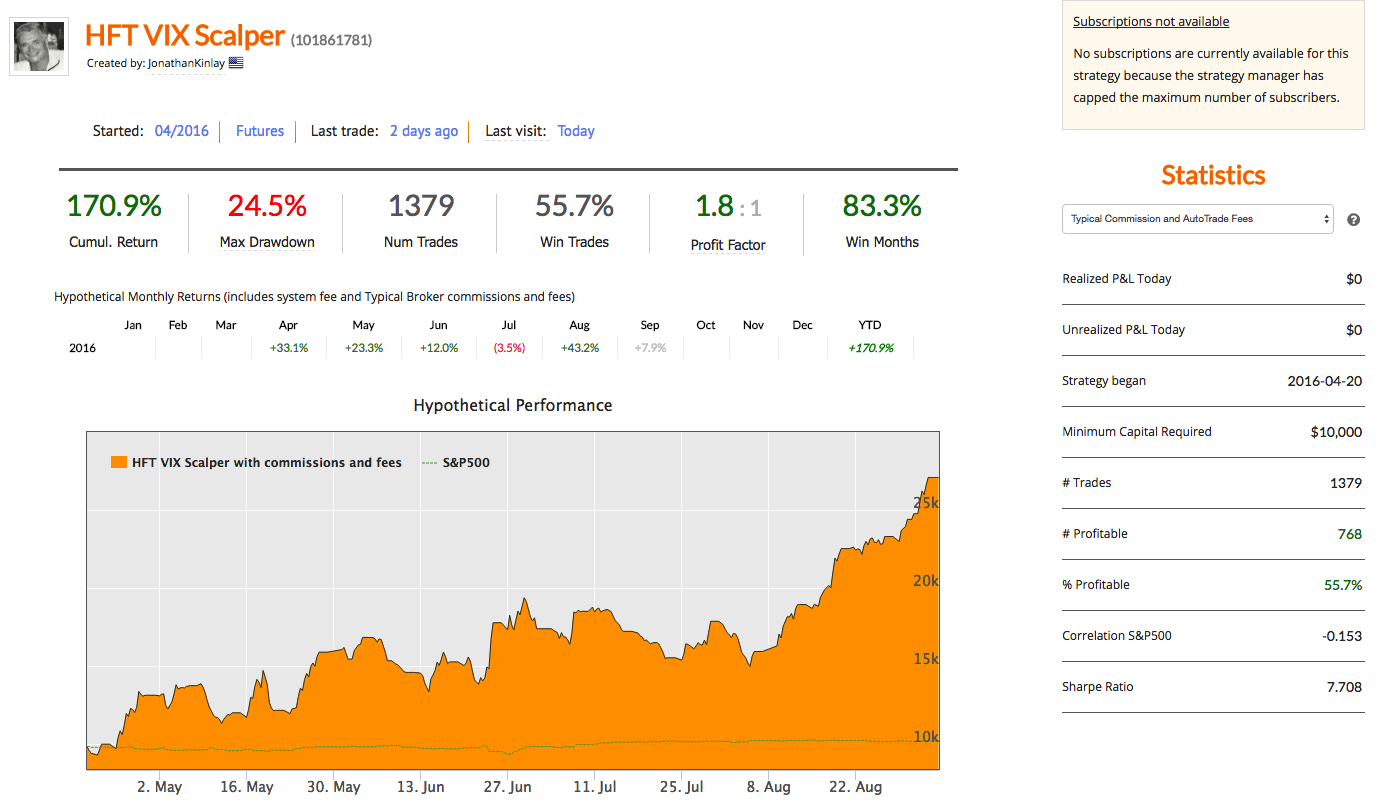
In my blog post Riders on the Storm I described one such approach: the Option Trader strategy on our Algo Trading Platform made a massive gain of 27% for the month of February and as a result strategy performance is now running at over 55% for 2018 YTD, while maintaining a Sharpe Ratio of 2.23.

The challenge with this style of volatility trading is that it requires a trader (or trading system) with a very strong stomach and an investor astute enough to realize that sizable drawdowns are in a sense “baked in” for this trading strategy and should be expected from time to time. But traders are often temperamentally unsuited to this style of trading – many react by heading for the hills and liquidating positions at the first sign of trouble; and the great majority of investors are likewise unable to withstand substantial drawdowns, even if the eventual outcome is beneficial.

The Market Timing Approach

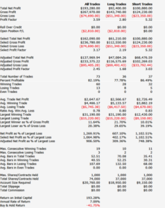
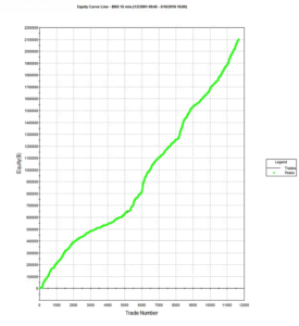
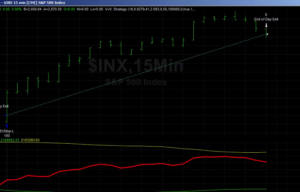
So what alternatives are there? One way of dealing with the problem of volatility spikes is simply to try to avoid them. That means developing a strategy logic that step aside altogether when there is a serious risk of an impending volatility surge. Market timing is easy to describe, but very hard to implement successfully in practice. The VIX Swing Trader strategy on the Systematic Algotrading platform attempts to do just that, only trading when it judges it safe to do so. So, for example, it completely side-stepped the volatility debacle in August 2015, ending the month up +0.74%. The strategy managed to do the same in February this year, finishing ahead +1.90%, a pretty creditable performance given how volatility funds performed in general. One helpful characteristic of the strategy is that it trades the less-volatile mid-section of the volatility curve, in the form of the VelocityShares Daily Inverse VIX MT ETN (ZIV). This ensures that the P&L swings are much less dramatic than for strategies exposed to the front end of the curve, as most volatility strategies are.

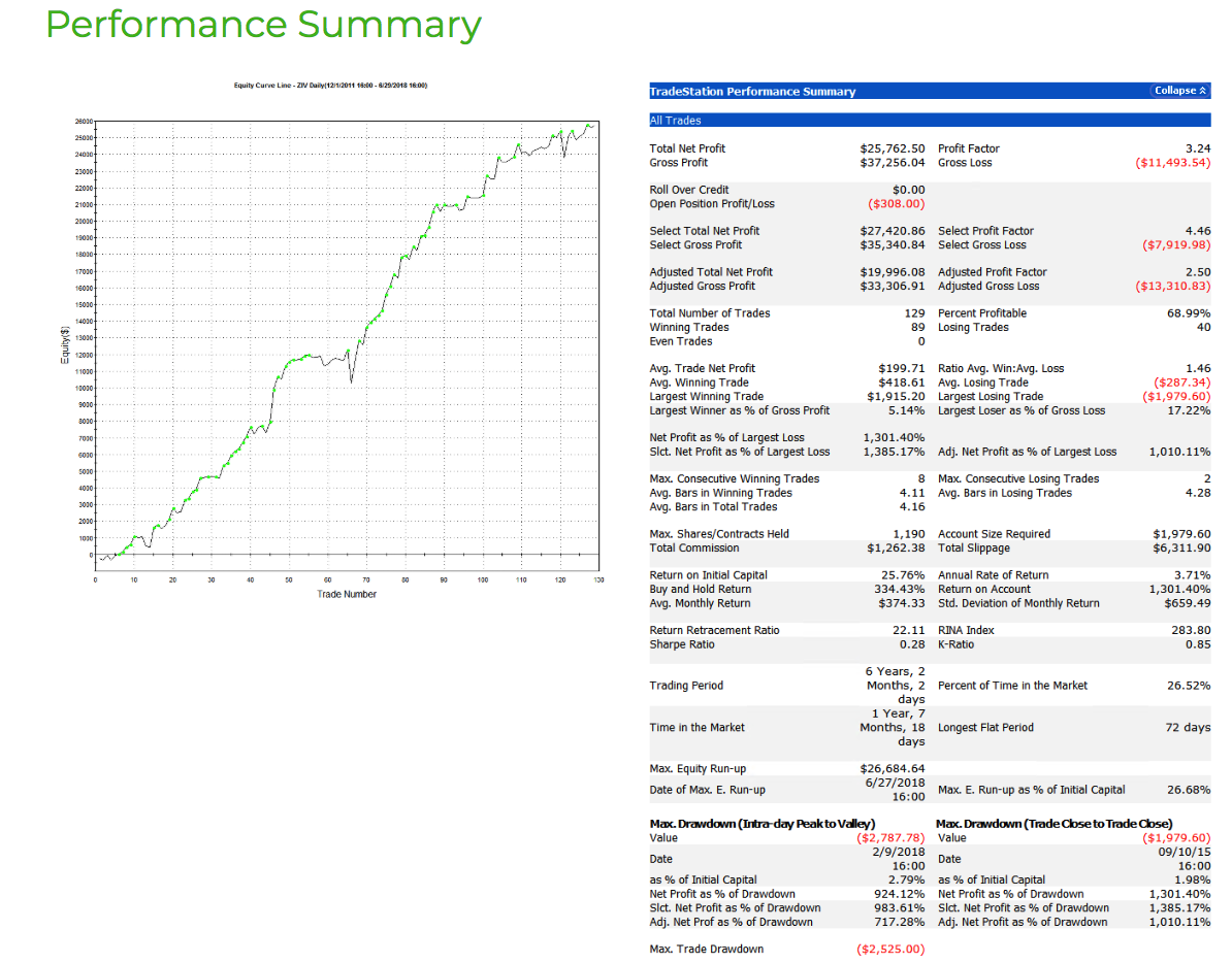
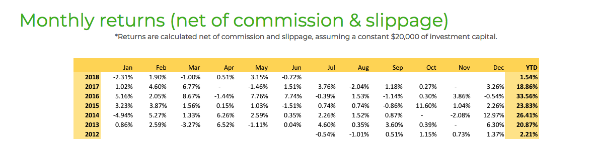
A potential weakness of the strategy is that it will often miss great profit opportunities altogether, since its primary focus is to keep investors out of trouble. Allied to this, the system may trade only a handful of times each month. Indeed, if you look at the track record above you find find months in which the strategy made no trades at all. From experience, investors are almost as bad at sitting on their hands as they are at taking losses: patience is not a highly regarded virtue in the investing community these days. But if you are a cautious, patient investor looking for a source of uncorrelated alpha, this strategy may be a good choice. On the other hand, if you are looking for high returns and are willing to take the associated risks, there are choices better suited to your goals.

The Hedging Approach to Volatility Trading

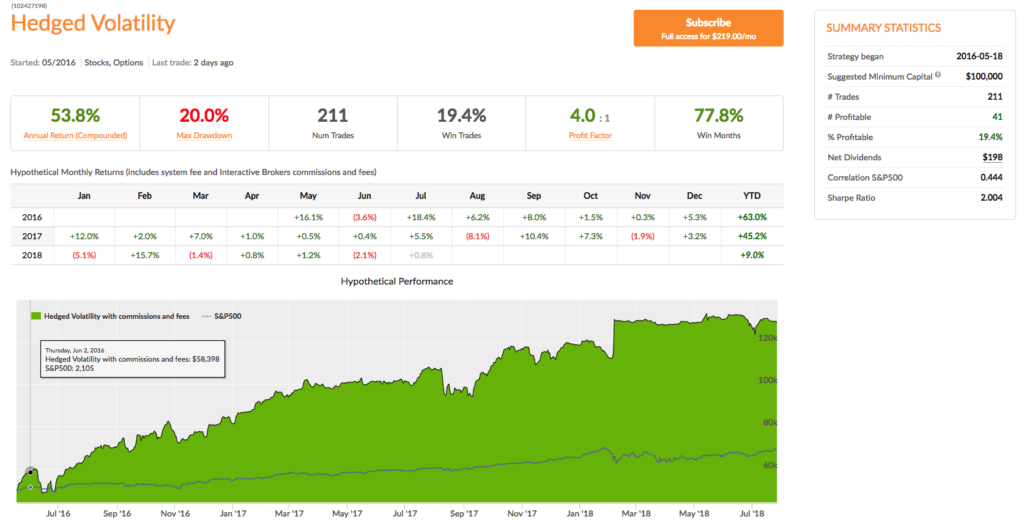
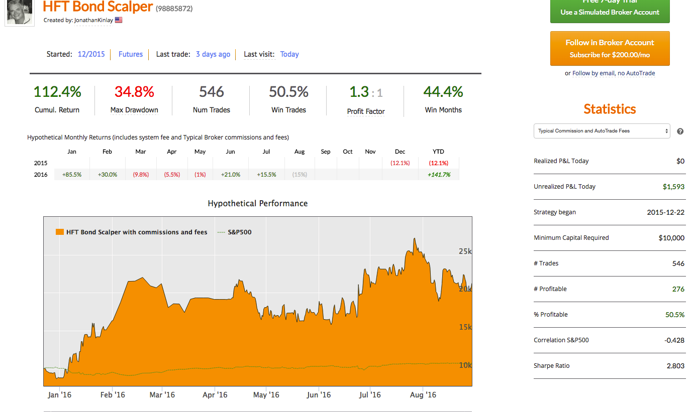
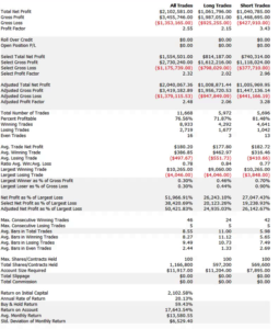
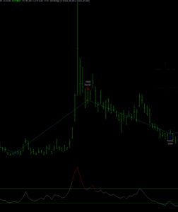
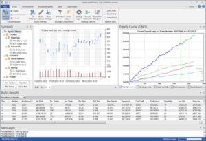
A “middle ground” is taken in our Hedged Volatility strategy. Like the VIX Swing Trader this strategy trades VIX ETFs/ETNs, but it does so across the maturity table. What distinguishes this strategy from the others is its use of long call options in volatility products like the iPath S&P 500 VIX ST Futures ETN (VXX) to hedge the short volatility exposure in other ETFs in the portfolio. This enables the strategy to trade much more frequently, across a wider range of ETF products and maturities, with the security of knowing that the tail risk in the portfolio is protected. Consequently, since live trading began in 2016, the strategy has chalked up returns of over 53% per year, with a Sharpe Ratio of 2 and Sortino Ratio above 3. Don’t be confused by the low % of trades that are profitable: the great majority of these loss-making “trades” are in fact hedges, which one would expect to be losers, as most long options trades are. What matters is the overall performance of the strategy.

All of these strategies are available on our Systematic Algotrading Platform, which offers investors the opportunity to trade the strategies in their own brokerage account for a monthly subscription fee.

The Multi-Strategy Approach

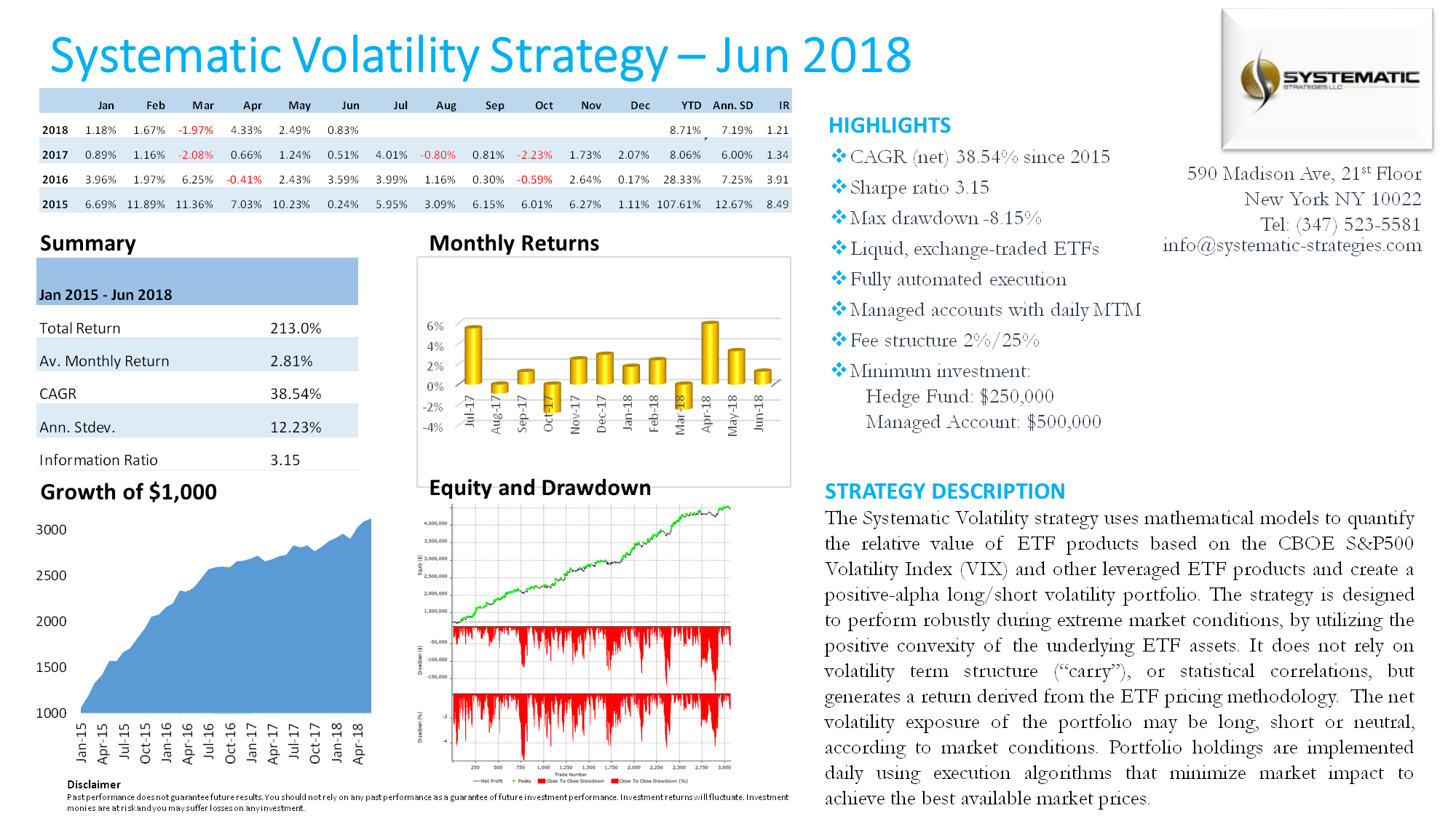
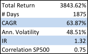
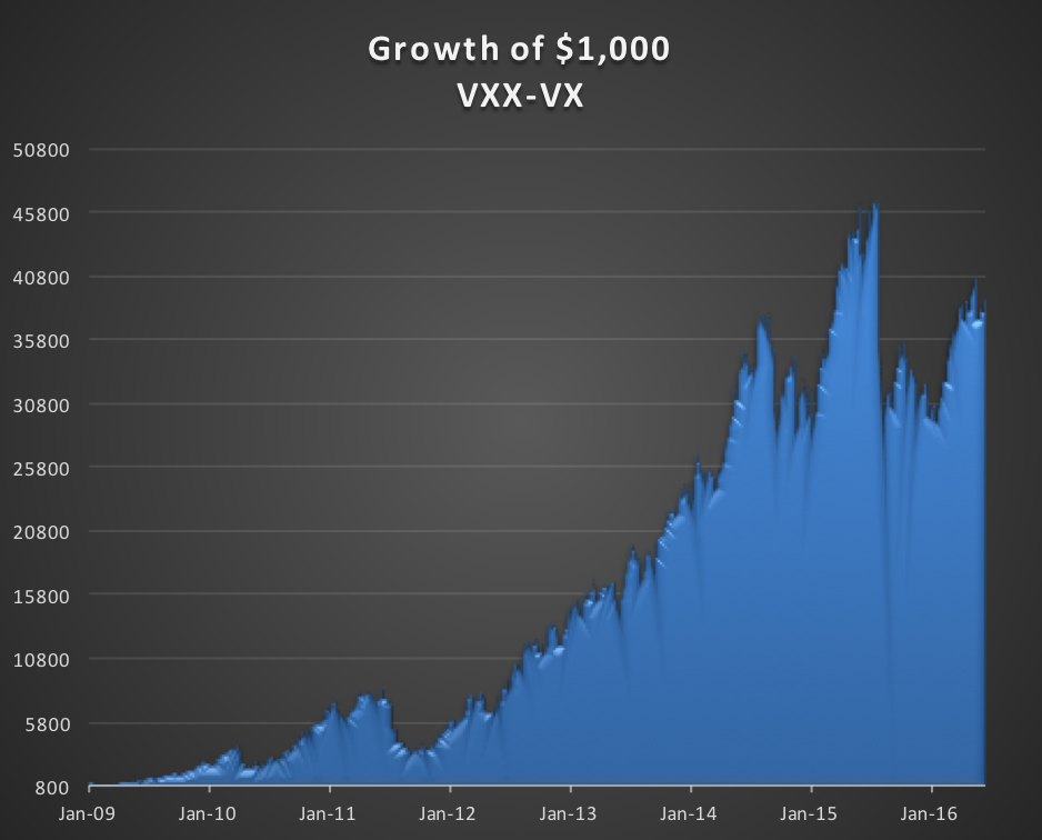
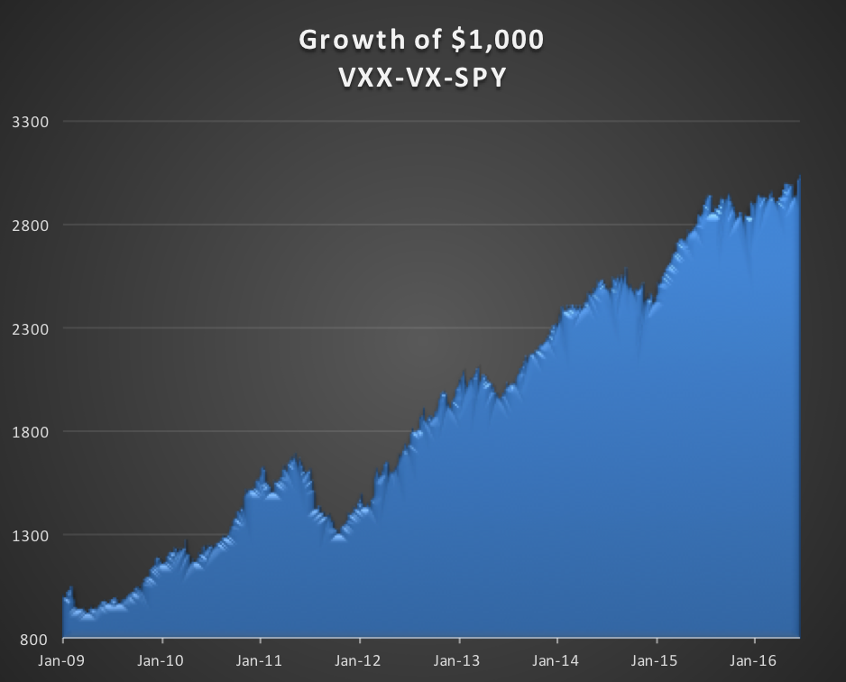
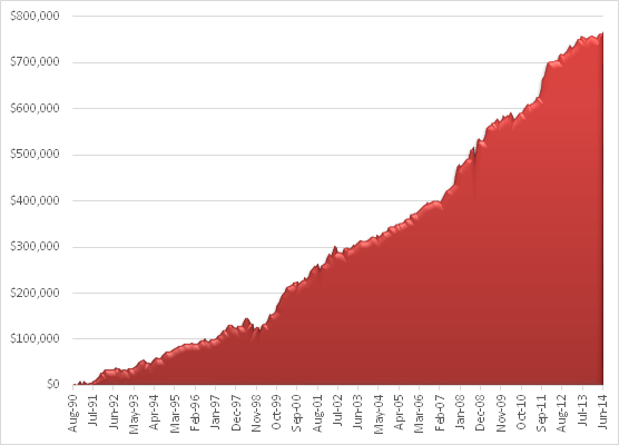
The approach taken by the Systematic Volatility Strategy in our Systematic Strategies hedge fund again seeks to steer a middle course between risk and return. It does so by using a meta-strategy approach that dynamically adjusts the style of strategy deployed as market conditions change. Rather than using options (the strategy’s mandate includes only ETFs) the strategy uses leveraged ETFs to provide tail risk protection in the portfolio. The strategy has produced an average annual compound return of 38.54% since live trading began in 2015, with a Sharpe Ratio of 3.15:

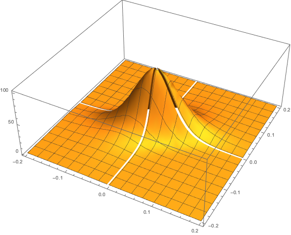
A more detailed explanation of how leveraged ETFs can be used in volatility trading strategies is given in an earlier post:

http://jonathankinlay.com/2015/05/investing-leveraged-etfs-theory-practice/

Conclusion: Choosing the Investment Style that’s Right for You

There are different styles of volatility trading and the investor should consider carefully which best suits his own investment temperament. For the “high risk” investor seeking the greatest profit the Option Trader strategy in an excellent choice, producing returns of +176% per year since live trading began in 2016. At the other end of the spectrum, the VIX Swing trader is suitable for an investor with a cautious trading style, who is willing to wait for the right opportunities, i.e. ones that are most likely to be profitable. For investors seeking to capitalize on opportunities in the volatility space, but who are concerned about the tail risk arising from major market corrections, the Hedge Volatility strategy offers a better choice. Finally, for investors able to invest $250,000 or more, a hedge fund investment in our Systematic Volatility strategy offers the highest risk-adjusted rate of return.

April 21, 2020

The Story of a HFT Strategy

VIX HFT Scalper

April 14, 2020April 14, 2020

Correlation Copulas

Continuing a previous post, in which we modeled the relationship in the levels of the VIX Index and the Year 1 and Year 2 CBOE Correlation Indices, we next turn our attention to modeling changes in the VIX index.

In case you missed it, the post can be found here:

http://jonathankinlay.com/2017/08/correlation-cointegration/

We saw previously that the levels of the three indices are all highly correlated, and we were able to successfully account for approximately half the variation in the VIX index using either linear regression models or non-linear machine-learning models that incorporated the two correlation indices. It turns out that the log-returns processes are also highly correlated:

A Linear Model of VIX Returns

We can create a simple linear regression model that relates log-returns in the VIX index to contemporaneous log-returns in the two correlation indices, as follows. The derived model accounts for just under 40% of the variation in VIX index returns, with each correlation index contributing approximately one half of the total VIX return.

Non-Linear Model of VIX Returns

Although the linear model is highly statistically significant, we see clear evidence of lack of fit in the model residuals, which indicates non-linearities present in the relationship. So, ext we use a nearest-neighbor algorithm, a machine learning technique that allows us to model non-linear components of the relationship. The residual plot from the nearest neighbor model clearly shows that it does a better job of capturing these nonlinearities, with lower standard in the model residuals, compared to the linear regression model:

Correlation Copulas

Another approach entails the use of copulas to model the inter-dependency between the volatility and correlation indices. For a fairly detailed exposition on copulas, see the following blog posts:

http://jonathankinlay.com/2017/01/copulas-risk-management/

http://jonathankinlay.com/2017/03/pairs-trading-copulas/

We begin by taking a smaller sample comprising around three years of daily returns in the indices. This minimizes the impact of any long-term nonstationarity in the processes and enables us to fit marginal distributions relatively easily. First, let’s look at the correlations in our sample data:

We next proceed to fit margin distributions to the VIX and Correlation Index processes. It turns out that the VIX process is well represented by a Logistic distribution, while the two Correlation Index returns processes are better represented by a Student-T density. In all three cases there is little evidence of lack of fit, wither in the body or tails of the estimated probability density functions:

The final step is to fit a copula to model the joint density between the indices. To keep it simple I have chosen to carry out the analysis for the combination of the VIX index with only the first of the correlation indices, although in principle there no reason why a copula could not be estimated for all three indices. The fitted model is a multinormal Gaussian copula with correlation coefficient of 0.69. of course, other copulas are feasible (Clayton, Gumbel, etc), but Gaussian model appears to provide an adequate fit to the empirical copula, with approximate symmetry in the left and right tails.

March 31, 2020

Correlation Cointegration

In a previous post I looked at ways of modeling the relationship between the CBOE VIX Index and the Year 1 and Year 2 CBOE Correlation Indices:

http://jonathankinlay.com/2017/08/modeling-volatility-correlation/

The question was put to me whether the VIX and correlation indices might be cointegrated.

Let’s begin by looking at the pattern of correlation between the three indices:

If you recall from my previous post, we were able to fit a linear regression model with the Year 1 and Year 2 Correlation Indices that accounts for around 50% in the variation in the VIX index. While the model certainly has its shortcomings, as explained in the post, it will serve the purpose of demonstrating that the three series are cointegrated. The standard Dickey-Fuller test rejects the null hypothesis of a unit root in the residuals of the linear model, confirming that the three series are cointegrated, order 1.

Vector Autoregression

We can attempt to take the modeling a little further by fitting a VAR model. We begin by splitting the data into an in-sample period from Jan 2007 to Dec 2015 and an out-of-sample test period from Jan 2016 to Aug 2017. We then fit a vector autoregression model to the in-sample data:

When we examine how the model performs on the out-of-sample data, we find that it fails to pick up on much of the variation in the series – the forecasts are fairly flat and provide quite poor predictions of the trends in the three series over the period from 2016-2017:

Conclusion

The VIX and Correlation Indices are not only highly correlated, but also cointegrated, in the sense that a linear combination of the series is stationary.

One can fit a weakly stationary VAR process model to the three series, but the fit is quite poor and forecasts from the model don’t appear to add much value. It is conceivable that a more comprehensive model involving longer lags would improve forecasting performance.

March 24, 2020

Modeling Volatility and Correlation

In a previous blog post I mentioned the VVIX/VIX Ratio, which is measured as the ratio of the CBOE VVIX Index to the VIX Index. The former measures the volatility of the VIX, or the volatility of volatility.

http://jonathankinlay.com/2017/07/market-stress-test-signals-danger-ahead/

A follow-up article in ZeroHedge shortly afterwards pointed out that the VVIX/VIX ratio had reached record highs, prompting Goldman Sachs analyst Ian Wright to comment that this could signal the ending of the current low-volatility regime:

A linkedIn reader pointed out that individual stock volatility was currently quite high and when selling index volatility one is effectively selling stock correlations, which had now reached historically low levels. I concurred:

What’s driving the low vol regime is the exceptionally low level of cross-sectional correlations. And, as correlations tighten, index vol will rise. Worse, we are likely to see a feedback loop – higher vol leading to higher correlations, further accelerating the rise in index vol. So there is a second order, Gamma effect going on. We see that is the very high levels of the VVIX index, which shot up to 130 last week. The all-time high in the VVIX prior to Aug 2015 was around 120. The intra-day high in Aug 2015 reached 225. I’m guessing it will get back up there at some point, possibly this year.

As there appears to be some interest in the subject I decided to add a further blog post looking a little further into the relationship between volatility and correlation. To gain some additional insight we are going to make use of the CBOE implied correlation indices. The CBOE web site explains:

Using SPX options prices, together with the prices of options on the 50 largest stocks in the S&P 500 Index, the CBOE S&P 500 Implied Correlation Indexes offers insight into the relative cost of SPX options compared to the price of options on individual stocks that comprise the S&P 500.

CBOE calculates and disseminates two indexes tied to two different maturities, usually one year and two years out. The index values are published every 15 seconds throughout the trading day.

Both are measures of the expected average correlation of price returns of S&P 500 Index components, implied through SPX option prices and prices of single-stock options on the 50 largest components of the SPX.

Dispersion Trading

One application is dispersion trading, which the CBOE site does a good job of summarizing:

The CBOE S&P 500 Implied Correlation Indexes may be used to provide trading signals for a strategy known as volatility dispersion (or correlation) trading. For example, a long volatility dispersion trade is characterized by selling at-the-money index option straddles and purchasing at-the-money straddles in options on index components. One interpretation of this strategy is that when implied correlation is high, index option premiums are rich relative to single-stock options. Therefore, it may be profitable to sell the rich index options and buy the relatively inexpensive equity options.

The VIX Index and the Implied Correlation Indices

Again, the CBOE web site is worth quoting:

The CBOE S&P 500 Implied Correlation Indexes measure changes in the relative premium between index options and single-stock options. A single stock’s volatility level is driven by factors that are different from what drives the volatility of an Index (which is a basket of stocks). The implied volatility of a single-stock option simply reflects the market’s expectation of the future volatility of that stock’s price returns. Similarly, the implied volatility of an index option reflects the market’s expectation of the future volatility of that index’s price returns. However, index volatility is driven by a combination of two factors: the individual volatilities of index components and the correlation of index component price returns.

Let’s dig into this analytically. We first download and plot the daily for the VIX and Correlation Indices from the CBOE web site, from which it is evident that all three series are highly correlated:

An inspection reveals significant correlations between the VIX index and the two implied correlation indices, which are themselves highly correlated. The S&P 500 Index is, of course, negatively correlated with all three indices:

Modeling Volatility-Correlation

The response surface that describes the relationship between the VIX index and the two implied correlation indices is locally very irregular, but the slope of the surface is generally positive, as we would expect, since the level of VIX correlates positively with that of the two correlation indices.

The most straightforward approach is to use a simple linear regression specification to model the VIX level as a function of the two correlation indices. We create a VIX Model Surface object using this specification with the Mathematica Predict function:The linear model does quite a good job of capturing the positive gradient of the response surface, and in fact has a considerable amount of explanatory power, accounting for a little under half the variance in the level of the VIX index:

However, there are limitations. To begin with, the assumption of independence between the explanatory variables, the correlation indices, clearly does not hold. In cases such as this, where explanatory variables are multicolinear, we are unable to draw inferences about the explanatory power of individual regressors, even though the model as a whole may be highly statistically significant, as here.

Secondly, a linear regression model is not going to capture non-linearities in the volatility-correlation relationship that are evident in the surface plot. This is confirmed by a comparison plot, which shows that the regression model underestimates the VIX level for both low and high values of the index:

We can achieve a better outcome using a machine learning algorithm such as nearest neighbor, which is able to account for non-linearities in the response surface:

The comparison plot shows a much closer correspondence between actual and predicted values of the VIX index, even though there is evidence of some remaining heteroscedasticity in the model residuals:

Conclusion

A useful way to think about index volatility is as a two dimensional process, with time-series volatility measured on one dimension and dispersion (cross-sectional volatility, the inverse of correlation) measured on the second. The two factors are correlated and, as we have shown here, interact in a complicated, non-linear way.

The low levels of index volatility we have seen in recent months result, not from low levels of volatility in component stocks, but in the historically low levels of correlation (high levels of dispersion) in the underlying stock returns processes. As correlations begin to revert to historical averages, the impact will be felt in an upsurge in index volatility, compounded by the non-linear interaction between the two factors.

November 12, 2019

HFT VIX Scalper Leads on Collective2

Our high frequency VIX scalping strategy is now the #1 top performing strategy on Collective2, with returns of over 2700% since April 2016 with a Sharpe Ratio above 10 and Profit Factor of 2.8.

For more background on HFT scalping strategies see the following post:

http://jonathankinlay.com/2014/05/the-mathematics-of-scalping/

September 17, 2019

High Frequency Futures Scalping Strategies Update

July 16, 2019

Developing A Volatility Carry Strategy

By way of introduction we begin by reviewing a well known characteristic of the iPath S&P 500 VIX ST Futures ETN (NYSEArca:VXX). In common with other long-volatility ETF /ETNs, VXX has a tendency to decline in value due to the upward sloping shape of the forward volatility curve. The chart below which illustrates the fall in value of the VXX, together with the front-month VIX futures contract, over the period from 2009.

This phenomenon gives rise to opportunities for “carry” strategies, wherein a long volatility product such as VXX is sold in expectation that it will decline in value over time. Such strategies work well during periods when volatility futures are in contango, i.e. when the longer dated futures contracts have higher prices than shorter dated futures contracts and the spot VIX Index, which is typically the case around 70% of the time. An analogous strategy in the fixed income world is known as “riding down the yield curve”. When yield curves are upward sloping, a fixed income investor can buy a higher-yielding bill or bond in the expectation that the yield will decline, and the price rise, as the security approaches maturity. Quantitative easing put paid to that widely utilized technique, but analogous strategies in currency and volatility markets continue to perform well.

The challenge for any carry strategy is what happens when the curve inverts, as futures move into backwardation, often giving rise to precipitous losses. A variety of hedging schemes have been devised that are designed to mitigate the risk. For example, one well-known carry strategy in VIX futures entails selling the front month contract and hedging with a short position in an appropriate number of E-Mini S&P 500 futures contracts. In this case the hedge is imperfect, leaving the investor the task of managing a significant basis risk.

The chart of the compounded value of the VXX and VIX futures contract suggests another approach. While both securities decline in value over time, the fall in the value of the VXX ETN is substantially greater than that of the front month futures contract. The basic idea, therefore, is a relative value trade, in which we purchase VIX futures, the better performing of the pair, while selling the underperforming VXX. Since the value of the VXX is determined by the value of the front two months VIX futures contracts, the hedge, while imperfect, is likely to entail less basis risk than is the case for the VIX-ES futures strategy.

Another way to think about the trade is this: by combining a short position in VXX with a long position in the front-month futures, we are in effect creating a residual exposure in the value of the second month VIX futures contract relative to the first. So this is a strategy in which we are looking to capture volatility carry, not at the front of the curve, but between the first and second month futures maturities. We are, in effect, riding down the belly of volatility curve.

The Relationship between VXX and VIX Futures

Let’s take a look at the relationship between the VXX and front month futures contract, which I will hereafter refer to simply as VX. A simple linear regression analysis of VXX against VX is summarized in the tables below, and confirms two features of their relationship.

Firstly there is a strong, statistically significant relationship between the two (with an R-square of 75% ) – indeed, given that the value of the VXX is in part determined by VX, how could there not be?

Secondly, the intercept of the regression is negative and statistically significant. We can therefore conclude that the underperformance of the VXX relative to the VX is not just a matter of optics, but is a statistically reliable phenomenon. So the basic idea of selling the VXX against VX is sound, at least in the statistical sense.

Constructing the Initial Portfolio

In constructing our theoretical portfolio, I am going to gloss over some important technical issues about how to construct the optimal hedge and simply assert that the best one can do is apply a beta of around 1.2, to produce the following outcome:

While broadly positive, with an information ratio of 1.32, the strategy performance is a little discouraging, on several levels. Firstly, the annual volatility, at over 48%, is uncomfortably high. Secondly, the strategy experiences very substantial drawdowns at times when the volatility curve inverts, such as in August 2015 and January 2016. Finally, the strategy is very highly correlated with the S&P500 index, which may be an important consideration for investors looking for ways to diversity their stock portfolio risk.

Exploiting Calendar Effects

We will address these issues in short order. Firstly, however, I want to draw attention to an interesting calendar effect in the strategy (using a simple pivot table analysis).

As you can see from the table above, the strategy returns in the last few days of the calendar month tend to be significantly below zero.

The cause of the phenomenon has to do with the way the VXX is constructed, but the important point here is that, in principle, we can utilize this effect to our advantage, by reversing the portfolio holdings around the end of the month. This simple technique produces a significant improvement in strategy returns, while lowering the correlation:

Reducing Portfolio Risk and Correlation

We can now address the issue of the residual high level of strategy volatility, while simultaneously reducing the strategy correlation to a much lower level. We can do this in a straightforward way by adding a third asset, the SPDR S&P 500 ETF Trust (NYSEArca:SPY), in which we will hold a short position, to exploit the negative correlation of the original portfolio.

We then adjust the portfolio weights to maximize the risk-adjusted returns, subject to limits on the maximum portfolio volatility and correlation. For example, setting a limit of 10% for both volatility and correlation, we achieve the following result (with weights -0.37 0.27 -0.65 for VXX, VX and SPY respectively):

Compared to the original portfolio, the new portfolio’s performance is much more benign during the critical period from Q2-2015 to Q1-2016 and while there remain several significant drawdown periods, notably in 2011, overall the strategy is now approaching an investable proposition, with an information ratio of 1.6 and annual volatility of 9.96% and correlation of 0.1.

Other configurations are possible, of course, and the risk-adjusted performance can be improved, depending on the investor’s risk preferences.

Portfolio Rebalancing

There is an element of curve-fitting in the research process as described so far, in as much as we are using all of the available data to July 2016 to construct a portfolio with the desired characteristics. In practice, of course, we will be required to rebalance the portfolio on a periodic basis, re-estimating the optimal portfolio weights as new data comes in. By way of illustration, the portfolio was re-estimated using in-sample data to the end of Feb, 2016, producing out-of-sample results during the period from March to July 2016, as follows:

A detailed examination of the generic problem of how frequently to rebalance the portfolio is beyond the scope of this article and I leave it to interested analysts to perform the research for themselves.

Practical Considerations

In order to implement the theoretical strategy described above there are several important practical steps that need to be considered.

It is not immediately apparent how the weights should be applied to a portfolio comprising both ETNs and futures. In practice the best approach is to re-estimate the portfolio using a regression relationship expressed in $-value terms, rather than in percentages, in order to establish the quantity of VXX and SPY stock to be sold per single VX futures contract.

Reversing the portfolio holdings in the last few days of the month will add significantly to transaction costs, especially for the position in VX futures, for which the minimum tick size is $50. It is important to factor realistic estimates of transaction costs into the assessment of the strategy performance overall and specifically with respect to month-end reversals.

The strategy assumed the availability of VXX and SPY to short, which occasionally can be a problem. It’s not such a big deal if you are maintaining a long-term short position, but flipping the position around over a few ays at the end of the month might be problematic, from time to time.

Also, we should take account of stock loan financing costs, which run to around 2.9% and 0.42% annually for VXX and SPY, respectively. These rates can vary with market conditions and stock availability, of course.

It is highly likely that other ETFs/ETNs could profitably be added to the mix in order to further reduce strategy volatility and improve risk-adjusted returns. Likely candidates could include, for example, the Direxion Daily 20+ Yr Trsy Bull 3X ETF (NYSEArca:TMF).

We have already mentioned the important issue of portfolio rebalancing. There is an argument for rebalancing more frequently to take advantage of the latest market data; on the other hand, too-frequent changes in the portfolio composition can undermine portfolio robustness, increase volatility and incur higher transaction costs. The question of how frequently to rebalance the portfolio is an important one that requires further testing to determine the optimal rebalancing frequency.

Conclusion

We have described the process of constructing a volatility carry strategy based on the relative value of the VXX ETN vs the front-month contract in VIX futures. By combining a portfolio comprising short positions in VXX and SPY with a long position in VIX futures, the investor can, in principle achieve risk-adjusted returns corresponding to an information ratio of around 1.6, or more. It is thought likely that further improvements in portfolio performance can be achieved by adding other ETFs to the portfolio mix.

June 18, 2019

Trading With Indices

In this post I want to discuss ways to make use of signals from relevant market indices in your trading. These signals can add value regardless of whether you trade algorithmically or manually. The techniques described here are one of the most widely applicable in the quantitative analyst’s arsenal.

Let’s motivate the discussion by looking an example of a simple trading system trading the VIX on weekly bars. Performance results for the system are summarized in the chart and table below. The system outperforms the buy and hold return by a substantial margin, with a profit factor of over 3 and a win rate exceeding 82%. What’s not to like?

Well, for one thing, this isn’t really a trading system – because the VIX Index itself isn’t tradable. So the performance results are purely notional (and, if you didn’t already notice, no slippage or commission is included).

It is very easy to build high-performing trading system in indices – because they are not traded products, index prices are often stale and tend to “follow” the price action in the equivalent traded market.

This particular system for the VIX Index took me less than ten minutes to develop and comprises only a few lines of code. The system makes use of a simple RSI indicator to decide when to buy or sell the index. I optimized the indicator parameters (separately for long and short) over the period to 2012, and tested it out-of-sample on the data from 2013-2016.

inputs:
Price( Close ) ,
Length( 14 ) ,
OverSold( 30 ) ;

variables:
RSIValue( 0 );

RSIValue = RSI( Price, Length );
if CurrentBar > 1 and RSIValue crosses over OverSold then
Buy ( !( “RsiLE” ) ) next bar at market;

The daily system I built for the S&P 500 Index is a little more sophisticated than the VIX model, and produces the following results.

Using Index Trading Systems

We have seen that its trivially easy to build profitable trading systems for index products. But since they can’t be traded, what’s the point?

The analyst might be tempted by the idea of using the signals generated by an index trading system to trade a corresponding market, such as VIX or eMini futures. However, this approach is certain to fail. Index prices lag the prices of equivalent futures products, where traders first monetize their view on the market. So using an index strategy directly to trade a cash or futures market would be like trying to trade using prices delayed by a few seconds, or minutes – a recipe for losing money.

Nor is it likely that a trading system developed for an index product will generalize to a traded market. What I mean by this is that if you were to take an index strategy, such as the VIX RSI strategy, transfer it to VIX futures and tweak the parameters in the hope of producing a profitable system, you are likely to be disappointed. As I have shown, you can produce a profitable index trading system using the simplest and most antiquated trading concepts (such as the RSI index) that long ago ceased to offer any predictive value in actual traded markets. Index markets are actually inefficient – the prices of index products often fail to fully reflect all relevant, available information in a timely way. Such simple inefficiencies are easily revealed by indicators such as moving averages. Traded markets, by contrast, are highly efficient and, with the exception of HFT, it is going to take a great deal more than a simple moving average to provide insight into the few inefficiencies that do arise.

Strategies in index products are best thought of, not as trading strategies, but rather as a means of providing broad guidance as to the general condition of the market and its likely direction over the longer term. To take the VIX index strategy as an example, you can see that each “trade” spans several weeks. So one might regard a “buy” signal from the VIX index system as an indication that volatility is expected to rise over the next month or two. A trader might use that information to lean on the side of being long volatility, perhaps even avoiding any short volatility positions altogether for the next several weeks. Following the model’s guidance in that way would would certainly have helped many equity and volatility traders during the market sell off during August 2015, for example:

The S&P 500 Index model is one I use to provide guidance as to market conditions for the current trading day. It is a useful input to my thinking as to how aggressive I want my trading models to be during the upcoming session. If the index model suggests a positive tone to the market, with muted volatility, I might be inclined to take a more aggressive stance. If the model starts trading to the short side, however, I am likely to want to be much more cautious. Yesterday (May 16, 2016), for example, the index model took an early long trade, providing confirmation of the positive tenor to the market and encouraging me to trade volatility to the short side more aggressively.

In general, I would tend to classify index trading systems as “decision support” tools that provide a means of shading opinion on the market, or perhaps providing a means of calibrating trading models to the anticipated market conditions. However, they can be used in a more direct way, short of actual trading. For example, one of our volatility trading systems uses the trading signals from a trading system designed for the VVIX volatility-of-volatility index. Another approach is to use the signals from an index trading system as an indicator of the market regime in a regime switching model.

Designing Index Trading Models

Whereas it is profitability that is typically the primary design criterion for an actual trading system, given the purpose of an index trading system there are other criteria that are at least as important.

It should be obvious from these few illustrations that you want to design your index model to trade less frequently than the system you are intending to trade live: if you are swing-trading the eminis on daily bars, it doesn’t help to see 50 trades a day from your index system. What you want is an indication as to whether the market action over the next several days is likely to be positive or negative. This means that, typically, you will design your index system using bar frequencies at least as long as for your live system.

Another way to slow down the signals coming from your index trading system is to design it for very high accuracy – a win rate of 70%, or higher. It is actually quite easy to do this: I have systems that trade the eminis on daily bars that have win rates of over 90%. The trick is simply that you have to be prepared to wait a long time for the trade to come good. For a live system that can often be a problem – no-one like to nurse an underwater position for days or weeks on end. But for an index trading system it matters far less and, in fact, it helps: because you want trading signals over longer horizons than the time intervals you are using in your live trading system.

Since the index system doesn’t have to trade live, it means of course that the usual trading costs and frictions do not apply. The advantage here is that you can come up with concepts for trading systems that would be uneconomic in the real world, but which work perfectly well in the frictionless world of index trading. The downside, however, is that this might lead you to develop index systems that trade far too frequently. So, even though they should not apply, you might seek to introduce trading costs in order to penalize higher frequency trading systems and benefit systems that trade less frequently.

Designing index trading systems in an area in which genetic programming algorithms excel. There are two main reasons for this. Firstly, as I have previously discussed, simple technical indicators of the kind employed by GP modeling systems work well in index markets. Secondly, and more importantly, you can use the GP system to tailor an index trading system to meet the precise criteria you have in mind, such as the % win rate, trading frequency, etc.

An outstanding product that I can highly recommend in this context is Mike Bryant’s Adaptrade Builder. Builder is a superb piece of software whose power and ease of use reflects Mike’s engineering background and systems development expertise.

September 12, 2018

How to Bulletproof Your Portfolio

Summary

How to stay in the market and navigate the rocky terrain ahead, without risking hard won gains.

A hedging program to get you out of trouble at the right time and step back in when skies are clear.

Even a modest ability to time the market can produce enormous dividends over the long haul.

Investors can benefit by using quantitative market timing techniques to strategically adjust their market exposure.

Market timing can be a useful tool to avoid major corrections, increasing investment returns, while reducing volatility and drawdowns.

The Role of Market Timing

Investors have enjoyed record returns since the market lows in March 2009, but sentiment is growing that we may be in the final stages of this extended bull run. The road ahead could be considerably rockier. How do you stay the course, without risking all those hard won gains?

The smart move might be to take some money off the table at this point. But there could be adverse tax effects from cashing out and, besides, you can’t afford to sit on the sidelines and miss another 3,000 points on the Dow. Hedging tools like index options, or inverse volatility plays such as the VelocityShares Daily Inverse VIX Short-Term ETN (NASDAQ:XIV), are too expensive. What you need is a hedging program that will get you out of trouble at the right time – and step back in when the skies are clear. We’re talking about a concept known as market timing.

Market timing is the ability to switch between risky investments such as stocks and less-risky investments like bonds by anticipating the overall trend in the market. It’s extremely difficult to do. But as Nobel prize-winning economist Robert C. Merton pointed out in the 1980s, even a modest ability to time the market can produce enormous dividends over the long haul. This is where quantitative techniques can help – regardless of the nature of your underlying investment strategy.

Let’s assume that your investment portfolio is correlated with a broad US equity index – we’ll use the SPDR S&P 500 Trust ETF (NYSEARCA:SPY) as a proxy, for illustrative purposes. While the market has more than doubled over the last 15 years, this represents a modest average annual return of only 7.21%, accompanied by high levels of volatility of 20.48% annually, not to mention sizeable drawdowns in 2000 and 2008/09.

Fig. 1 SPY – Value of $1,000 Jan 1999 – Jul 2014

Source: Yahoo! Finance, 2014

The aim of market timing is to smooth out the returns by hedging, and preferably avoiding altogether, periods of market turmoil. In other words, the aim is to achieve the same, or better, rates of return, with lower volatility and drawdown.

Market Timing with the VIX Index

The mechanism we are going to use for timing our investment is the CBOE VIX index, a measure of anticipated market volatility in the S&P 500 index. It is well known that the VIX and S&P 500 indices are negatively correlated – when one rises, the other tends to fall. By acting ahead of rising levels of the VIX index, we might avoid difficult market conditions when market volatility is high and returns are likely to be low. Our aim would be to reduce market exposure during such periods and increase exposure when the VIX is in decline.

Forecasting the VIX index is a complex topic in its own right. The approach I am going to take here is simpler: instead of developing a forecasting model, I am going to use an algorithm to “trade” the VIX index. When the trading model “buys” the VIX index, we will assume it is anticipating increased market volatility and lighten our exposure accordingly. When the model “sells” the VIX, we will increase market exposure.

Don’t be misled by the apparent simplicity of this approach: a trading algorithm is often much more complex in its structure than even a very sophisticated forecasting model. For example, it can incorporate many different kinds of non-linear behavior and dynamically adjust its investment horizon. The results from such a trading algorithm, produced by our quantitative modeling system, are set out in the figure below.

Fig. 2a -VIX Trading Algorithm – Equity Curve

Source: TradeStation Technologies Inc.

Fig. 2b -VIX Trading Algorithm – Performance Analysis

Source: TradeStation Technologies Inc.

Not only is the strategy very profitable, it has several desirable features, including a high percentage of winning trades. If this were an actual trading system, we might want to trade it in production. But, of course, it is only a theoretical model – the VIX index itself is not tradable – and, besides, the intention here is not to trade the algorithm, but to use it for market timing purposes.

Our approach is straightforward: when the algorithm generates a “buy” signal in the VIX, we will reduce our exposure to the market. When the system initiates a “sell”, we will increase our market exposure. Trades generated by the VIX algorithm are held for around five days on average, so we can anticipate rebalancing our portfolio approximately weekly. In what follows, we will assume that we adjust our position by trading the SPY ETF at the closing price the day following a signal from the VIX model. We will apply trading commissions of $1c per share and a further $1c per share in slippage.

Hedging Strategies

Let’s begin our evaluation by looking at the outcome if we adjust the SPY holding in our market portfolio by 20% whenever the VIX model generates a signal. When the model buys the VIX, we will reduce our original SPY holding by 20%, and when it sells the VIX, we will increase our SPY holding by 20%, using the original holding in the long only portfolio as a baseline. We refer to this in the chart below as the MT 20% hedge portfolio.

Fig. 3 Value of $1000 – Long only vs MT 20% hedge portfolio

Source: Yahoo! Finance, 2014

The hedge portfolio dominates the long only portfolio over the entire period from 1999, producing a total net return of 156% compared to 112% for the SPY ETF. Not only is the rate of return higher, at 10.00% vs. 7.21% annually, volatility in investment returns is also significantly reduced (17.15% vs 20.48%). Although it, too, suffers substantial drawdowns in 2000 and 2008/09, the effects on the hedge portfolio are less severe. It appears that our market timing approach adds value.

The selection of 20% as a hedge ratio is somewhat arbitrary – an argument can be made for smaller, or larger, hedge adjustments. Let’s consider a different scenario, one in which we exit our long-only position entirely, whenever the VIX algorithm issues a buy order. We will re-buy our entire original SPY holding whenever the model issues a sell order in the VIX. We refer to this strategy variant as the MT cash out portfolio. Let’s look at how the results compare.

Fig. 4 Value of $1,000 – Long only vs MT cash out portfolio

Source: Yahoo! Finance, 2014

The MT cash out portfolio appears to do everything we hoped for, avoiding the downturn of 2000 almost entirely and the worst of the market turmoil in 2008/09. Total net return over the period rises to 165%, with higher average annual returns of 10.62%. Annual volatility of 9.95% is less than half that of the long only portfolio.

Finally, let’s consider a more extreme approach, which I have termed the “MT aggressive portfolio”. Here, whenever the VIX model issues a buy order we sell our entire SPY holding, as with the MT cash out strategy. Now, however, whenever the model issues a sell order on the VIX, we invest heavily in the market, buying double our original holding in SPY (i.e. we are using standard, reg-T leverage of 2:1, available to most investors). In fact, our average holding over the period turns out to be slightly lower than for the original long only portfolio because we are 100% in cash for slightly more than half the time. But the outcome represents a substantial improvement.

Fig. 5 Value of $1,000 – Long only vs. MT aggressive portfolio

Source: Yahoo! Finance, 2014

Total net returns for the MT aggressive portfolio at 330% are about three times that of the original long only portfolio. Annual volatility at 14.90% is greater than for the MT cash out portfolio due to the use of leverage. But this is still significantly lower than the 20.48% annual volatility of the long only portfolio, while the annual rate of return of 21.16% is the highest of the group, by far. And here, too, the hedge strategy succeeds in protecting our investment portfolio from the worst of the effects of downturns in 2000 and 2008.

Conclusion

Whatever the basis for their underlying investment strategy, investors can benefit by using quantitative market timing techniques to strategically adjust their market exposure. Market timing can be a useful tool to avoid major downturns, increasing investment returns while reducing volatility. This could be especially relevant in the weeks and months ahead, as we may be facing a period of greater uncertainty and, potentially at least, the risk of a significant market correction.

Disclosure: The author has no positions in any stocks mentioned, and no plans to initiate any positions within the next 72 hours. The author wrote this article themselves, and it expresses their own opinions. The author is not receiving compensation for it (other than from Seeking Alpha). The author has no business relationship with any company whose stock is mentioned in this article.