SPY Archives - QUANTITATIVE RESEARCH AND TRADING

March 13, 2024March 13, 2024

The Misunderstood Art of Market Timing:

How to Beat Buy-and-Hold with Less Risk

What is Market Timing? – Common Misconceptions

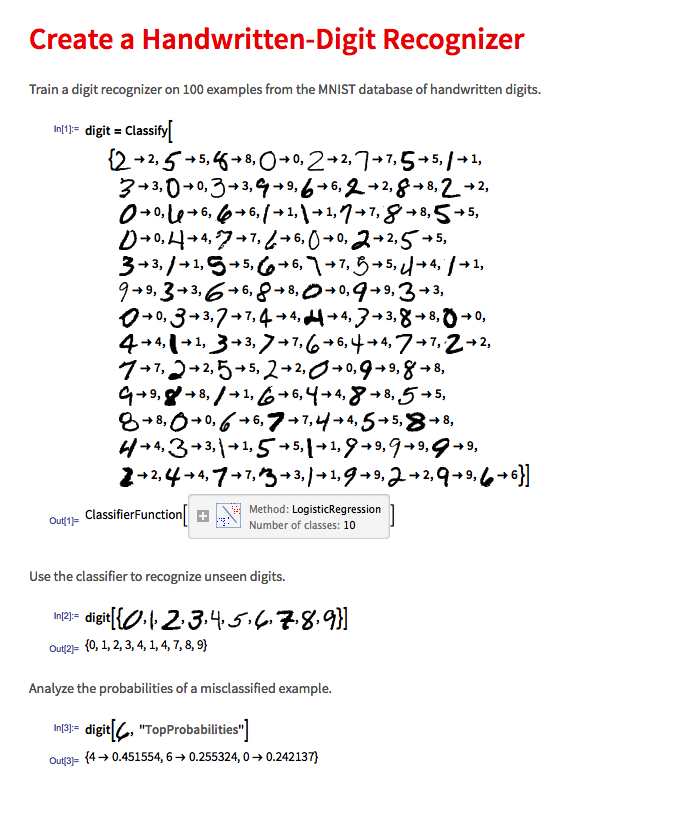
Market timing has a very bad press and for good reason: the inherent randomness of markets makes reliable forecasting virtually impossible. So why even bother to write about it? The answer is, because market timing has been mischaracterized and misunderstood. It isn’t about forecasting. If fact, with notable exceptions, most of trading isn’t about forecasting. It’s about conditional expectations.

Conditional expectations refer to the expected value of a random variable (such as future stock returns) given certain known information or conditions.

In the context of trading and market timing, it means that rather than attempting to forecast absolute price levels, we base our expectations for future returns on current observable market conditions.

For example, let’s say historical data shows that when the market has declined a certain percentage from its recent highs (condition), forward returns over the next several days tend to be positive on average (expectation). A trading strategy could use this information to buy the dip when that condition is met, not because it is predicting that the market will rally, but because history suggests a favorable risk/reward ratio for that trade under those specific circumstances.

The key insight is that by focusing on conditional expectations, we don’t need to make absolute predictions about where the market is heading. We simply assess whether the present conditions have historically been associated with positive expected returns, and use that probabilistic edge to inform our trading decisions.

This is a more nuanced and realistic approach than binary forecasting, as it acknowledges the inherent uncertainty of markets while still allowing us to make intelligent, data-driven decisions. By aligning our trades with conditional expectations, we can put the odds in our favor without needing a crystal ball.

So, when a market timing algorithm suggests buying the market, it isn’t making a forecast about what the market is going to do next. Rather, what it is saying is, if the market behaves like this then, on past experience, the following trade is likely to be profitable. That is a very different thing from forecasting the market.

A good example of a simple market-timing algorithm is “buying the dips”. It’s so simple that you don’t need a computer algorithm to do it. But a computer algorithm helps by determining what comprises a dip and the level at which profits should be taken.

An Effective Market Timing Strategy

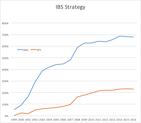
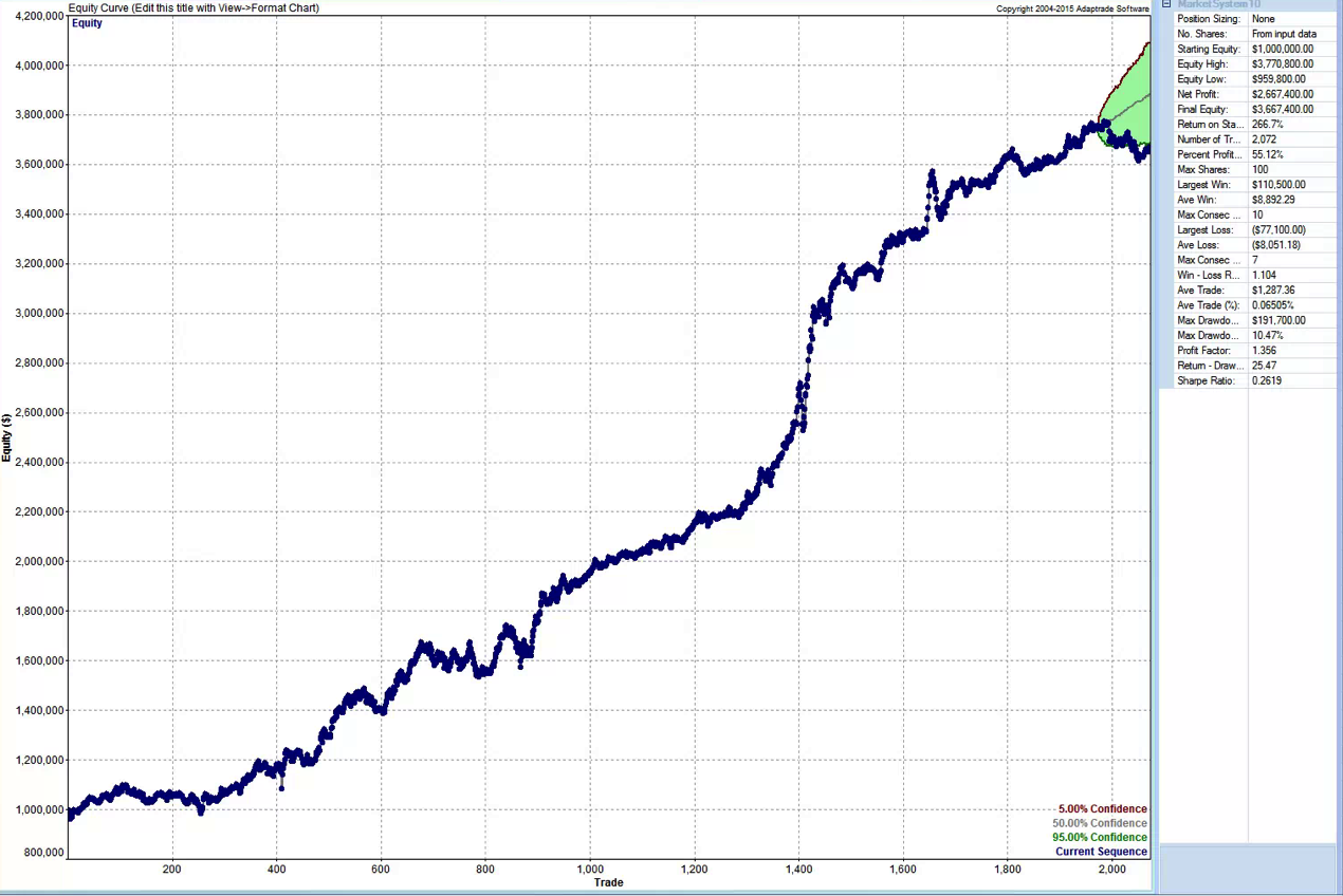
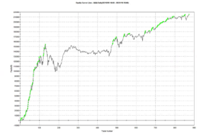
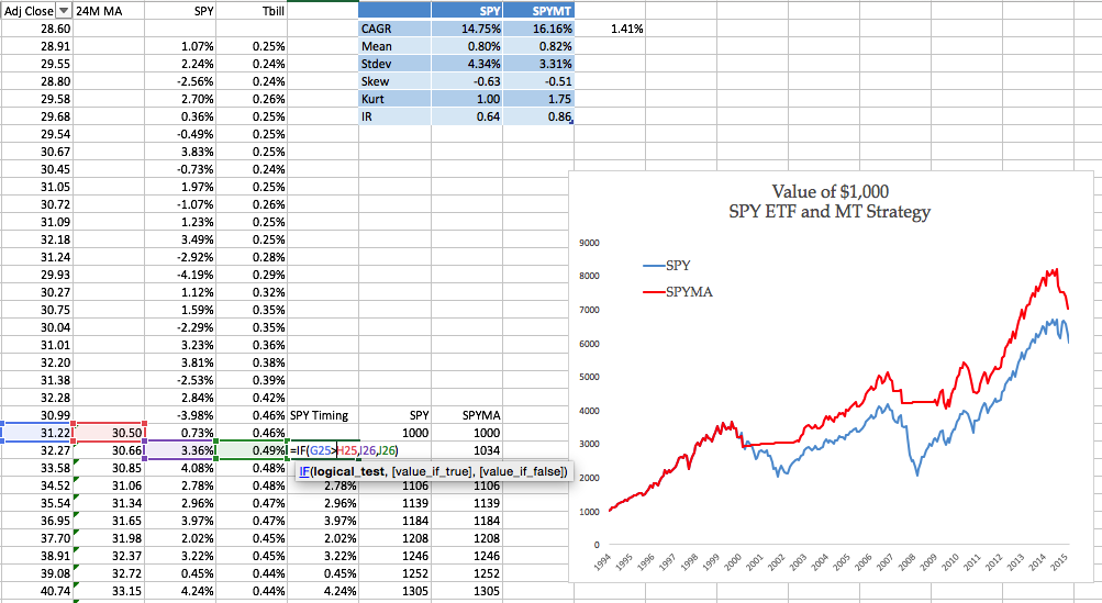
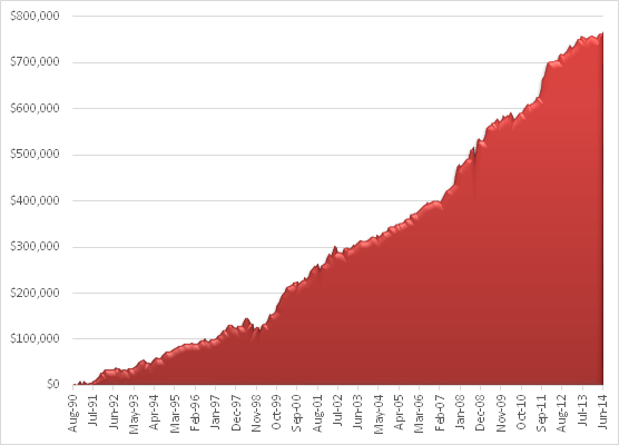
One of my favorites market timing strategies is the following algorithm, which I originally developed to trade the SPY ETF. The equity curve from inception of the ETF in 1993 looks like this:

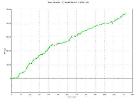
The algorithm combines a few simple technical indicators to determine what constitutes a dip and the level at which profits should be taken. The entry and exit orders are also very straightforward, buying and selling at the market open, which can be achieved by participating in the opening auction. This is very convenient: a signal is generated after the close on day 1 and is then executed as a MOA (market opening auction) order in the opening auction on day 2. The opening auction is by no means the most liquid period of the trading session, but in an ETF like SPY the volumes are such that the market impact is likely to be negligible for the great majority of investors. This is not something you would attempt to do in an illiquid small-cap stock, however, where entries and exits are more reliably handled using a VWAP algorithm; but for any liquid ETF or large-cap stock the opening auction will typically be fine.

Adapting the Strategy to Other Assets and Markets

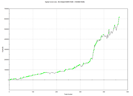
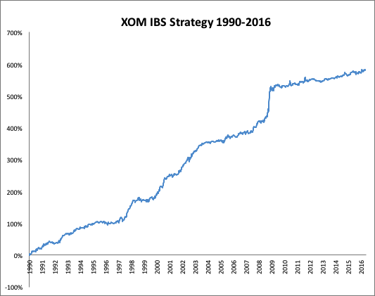
Another aspect that gives me confidence in the algorithm is that it generalizes well to other assets and even other markets. Here, for example, is the equity curve for the exact same algorithm implemented in the XLG ETF in the period from 2010:

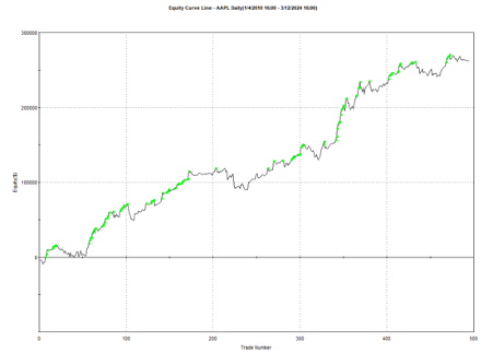
And here is the equity curve for the same strategy (with the same parameters) in AAPL, over the same period:

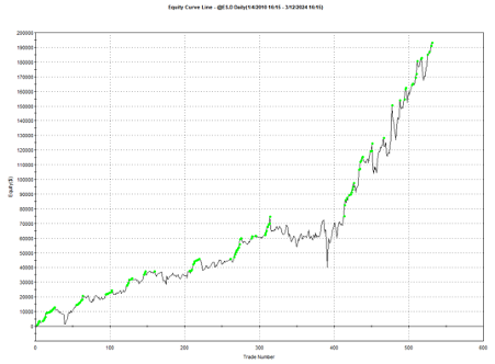
Remarkably, the strategy also works in E-mini futures too, which is highly unusual: typically the market dynamics of the futures market are so different from the spot market that strategies don’t transfer well. But in this case, it simply works:

Understanding Why the Strategy Works

The reason the strategy is effective is due to the upward drift in equities and related derivatives. If you tried to apply a similar strategy to energy or currency markets, it would fail. The strategy’s “secret sauce” is the combination of indicators it uses to determine the short-term low in the ETF that constitutes a good buying opportunity, and then figure out the right level at which to sell.

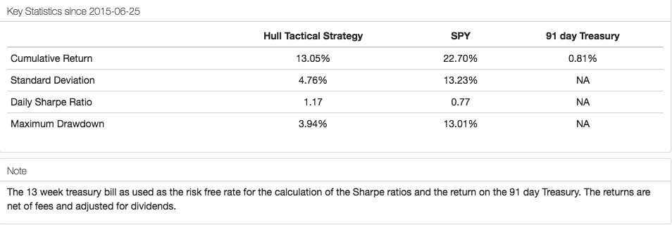
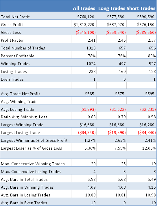
Does the algorithm always work? If by that you mean “is every trade profitable?” the answer is no. Around 61% of trades are profitable, so there are many instances where trades are closed at a loss. But the net impact of using the market-timing algorithm is very positive, when compared to the buy-and-hold benchmark, as we shall see shortly.

Because the underlying thesis is so simple (i.e. equity markets have positive drift), we can say something about the long-term prospects for the strategy. Equity markets haven’t changed their fundamental tendency to appreciate over the 31-year period from inception of the SPY ETF in 1993, which is why the strategy has performed well throughout that time. Could one envisage market conditions in which the strategy will perform poorly? Yes – any prolonged period of flat to downward trending prices in equities will result in poor performance. But we haven’t seen those conditions since the early 1970’s and, arguably, they are unlikely to return, since the fundamental change brought about by abandonment of the gold standard in 1973.

The abandonment of the gold standard and the subsequent shift to fiat currencies has given central banks, particularly the U.S. Federal Reserve, unprecedented power to expand the money supply and support asset prices during times of crisis. This ‘Fed Put’ has been a major factor underpinning the multi-decade bull market in stocks.

In addition, the increasing dominance of the U.S. as the world’s primary economic and military superpower since the end of the Cold War has made U.S. financial assets a uniquely attractive destination for global capital, creating sustained demand for U.S. equities.

Technological innovation, particularly with respect to the internet and advances in computing, has also unleashed a wave of productivity and wealth creation that has disproportionately benefited the corporate sector and equity holders. This trend shows no signs of abating and may even be accelerating with the advent of artificial intelligence.

While risks certainly remain and occasional cyclical bear markets are inevitable, the combination of accommodative monetary policy, the U.S.’s global hegemony, and technological progress create a powerful set of economic forces that are likely to continue propelling equity prices higher over the long-term, albeit with significant volatility along the way.Strategy Performance in Bear Markets

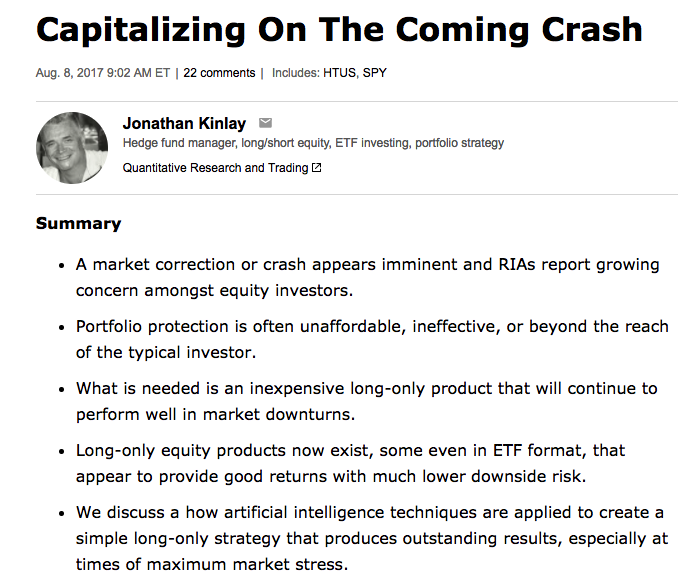
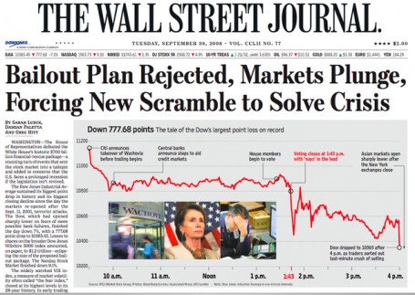
Note that the conditions I am referring to are something unlike anything we have seen in the last 50 years, not just a (serious) market pullback. If we look at the returns in the period from 2000-2002, for example, we see that the strategy held up very well, out-performing the benchmark by 54% over the three-year period of the market crash. Likewise, in 2008 credit crisis, the strategy was able to eke out a small gain, beating the benchmark by over 38%. In fact, the strategy is positive in all but one of the 31 years from inception.

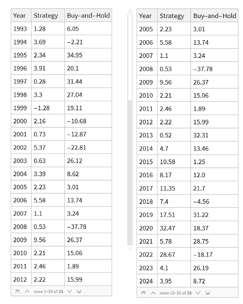
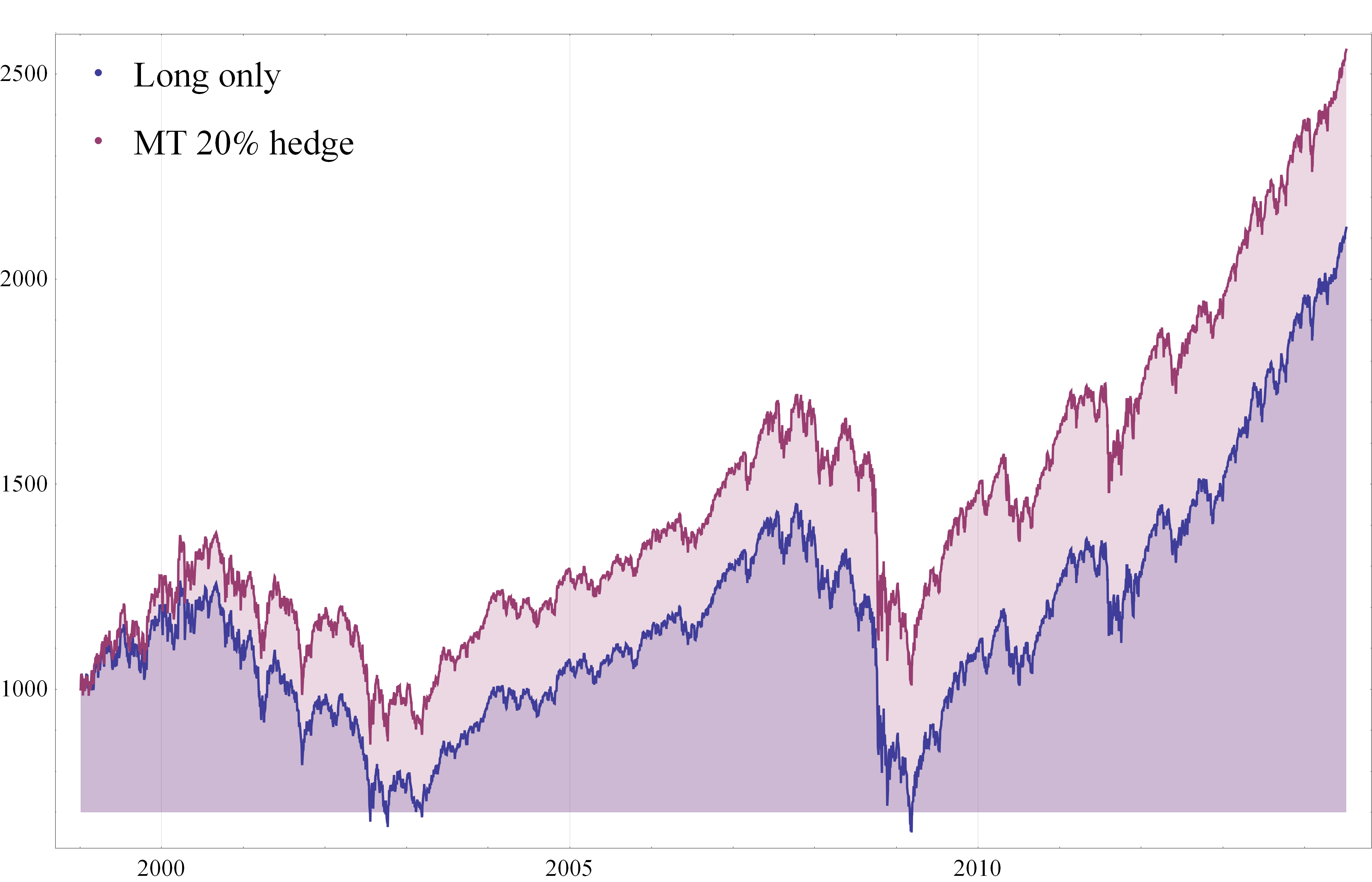
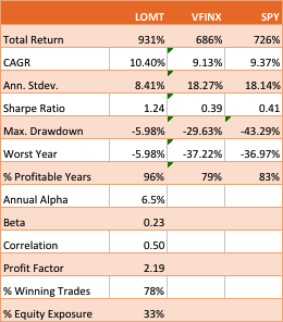
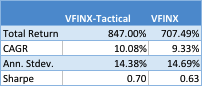
Comparing Performance to Buy-and-Hold

Let’s take a look at the compound returns from the strategy vs. the buy-and-hold benchmark:

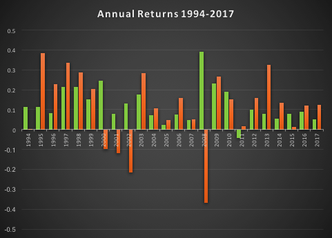
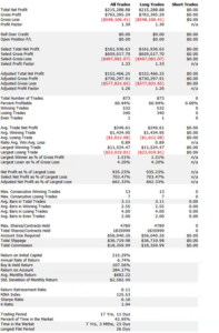
At first sight, it appears that the benchmark significantly out-performs the strategy, albeit suffering from much larger drawdowns. But that doesn’t give an accurate picture of relative performance. To see why, let’s look at the overall performance characteristics:

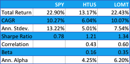
Now we see that, while the strategy CAGR is 3.50% below the buy-and-hold return, its annual volatility is less than half that of the benchmark, giving the strategy a superior Sharpe Ratio.

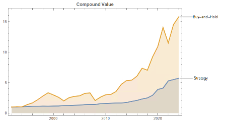
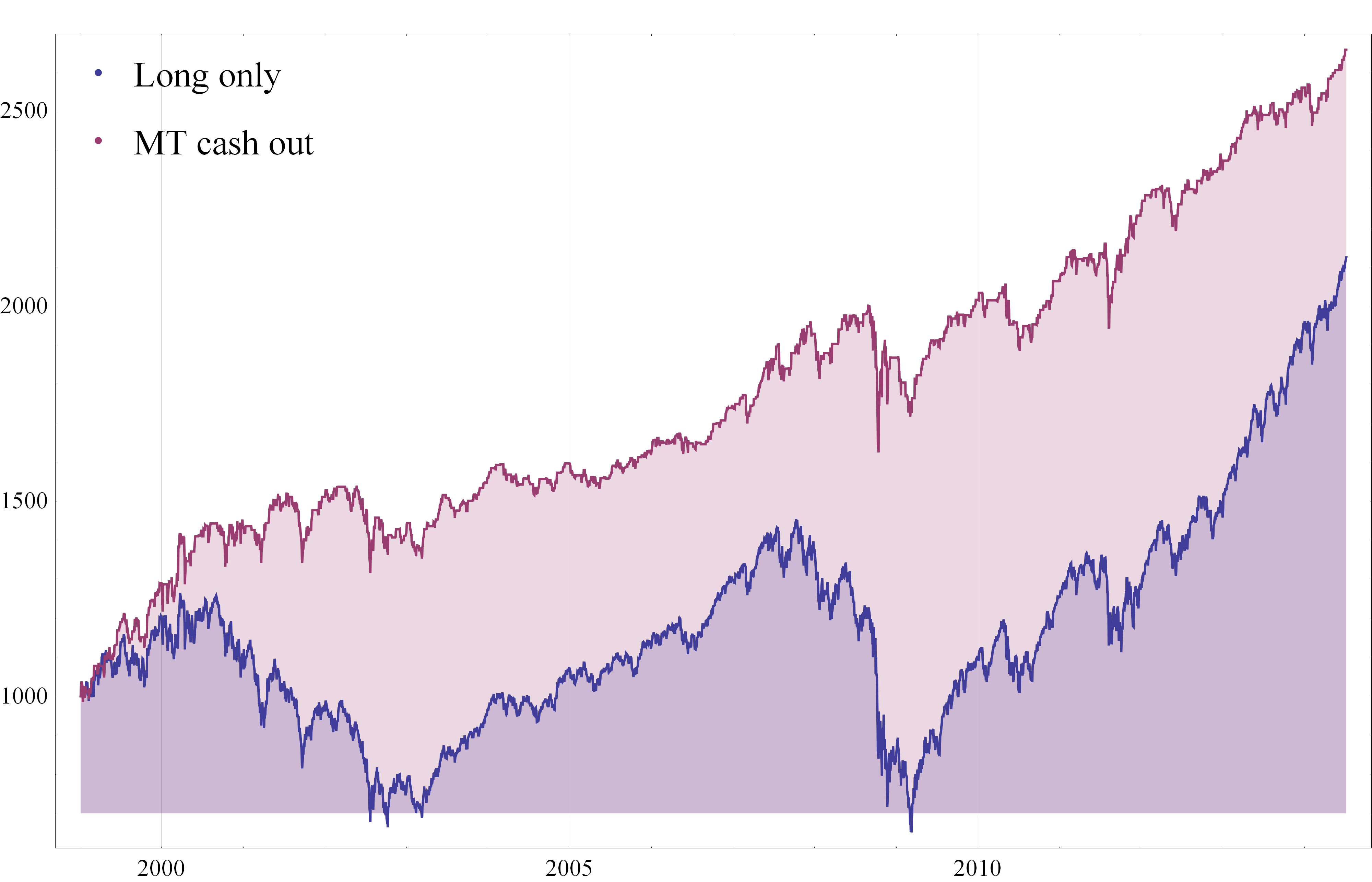
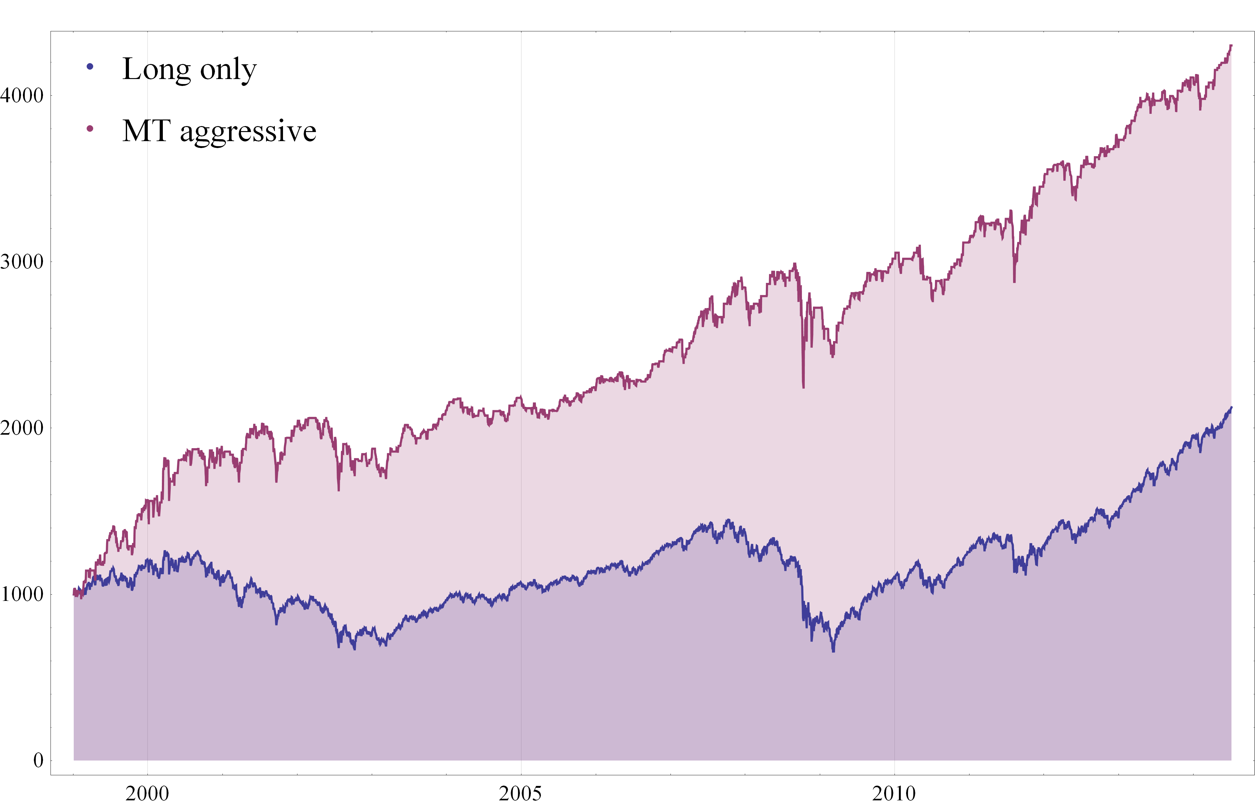
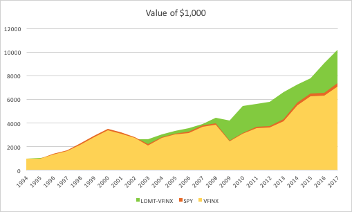
Leveraging the Strategy to Enhance Risk-Adjusted Returns

To make a valid comparison between the strategy and its benchmark we therefore need to equalize the annual volatility of both, and we can achieve this by leveraging the strategy by a factor of approximately 2.32. When we do that, we obtain the following results:

Now that the strategy and benchmark volatilities have been approximately equalized through leverage, we see that the strategy substantially outperforms buy-and-hold by around 355 basis points per year and with far smaller drawdowns.

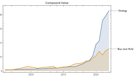
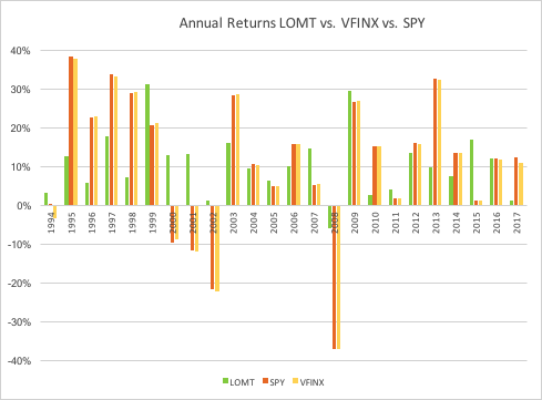
In general, we see that the strategy outperformed the benchmark in fewer than 50% of annual periods since 1993. However, the size of the outperformance in years when it beat the benchmark was frequently very substantial:

Conclusion

Market timing can work. To understand why, we need to stop thinking in terms of forecasting and think instead about conditional returns. When we do that, we arrive at the insight that market timing works because it relies on the positive drift in equity markets, which has been one of the central features of that market over the last 50 years and is likely to remain so in the foreseeable future. We have confidence in that prediction, because we understand the economic factors that have continued to drive the upward drift in equities over the last half-century.

After that, it is simply a question of the mechanics – how to time the entries and exits. This article describes just one approach amongst a great number of possibilities.

One of the many benefits of market timing is that it has a tendency to side-step the worst market conditions and can produce positive returns even in the most hostile environments: periods such as 2000-2002 and 2008, for example, as we have seen.

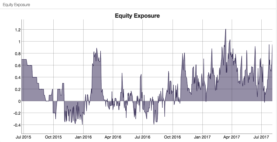
Finally, don’t forget that, as we are sitting out of the market approximately 40% of the time our overall risk is much lower – less than half that of the benchmark. So, we can afford to leverage our positions without taking on more overall risk than when we buy and hold. This clearly demonstrates the ability of the strategy to produce higher rates of risk-adjusted return.

March 17, 2020March 17, 2020

Tactical Mutual Fund Strategies

A recent blog post of mine was posted on Seeking Alpha (see summary below if you missed it).

The essence of the idea is simply that one can design long-only, tactical market timing strategies that perform robustly during market downturns, or which may even be positively correlated with volatility. I used the example of a LOMT (“Long-Only Market-Timing”) strategy that switches between the SPY ETF and 91-Day T-Bills, depending on the current outlook for the market as characterized by machine learning algorithms. As I indicated in the article, the LOMT handily outperforms the buy-and-hold strategy over the period from 1994 -2017 by several hundred basis points:

Of particular note is the robustness of the LOMT strategy performance during the market crashes in 2000/01 and 2008, as well as the correction in 2015:

The Pros and Cons of Market Timing (aka “Tactical”) Strategies

One of the popular choices the investor concerned about downsize risk is to use put options (or put spreads) to hedge some of the market exposure. The problem, of course, is that the cost of the hedge acts as a drag on performance, which may be reduced by several hundred basis points annually, depending on market volatility. Trying to decide when to use option insurance and when to maintain full market exposure is just another variation on the market timing problem.

The point of tactical strategies is that, unlike an option hedge, they will continue to produce positive returns – albeit at a lower rate than the market portfolio – during periods when markets are benign, while at the same time offering much superior returns during market declines, or crashes. If the investor is concerned about the lower rate of return he is likely to achieve during normal years, the answer is to make use of leverage.

Market timing strategies like Hull Tactical or the LOMT have higher risk-adjusted rates of return (Sharpe Ratios) than the market portfolio. So the investor can make use of margin money to scale up his investment to about the same level of risk as the market index. In doing so he will expect to earn a much higher rate of return than the market.

This is easy to do with products like LOMT or Hull Tactical, because they make use of marginable securities such as ETFs. As I point out in the sections following, one of the shortcomings of applying the market timing approach to mutual funds, however, is that they are not marginable (not initially, at least), so the possibilities for using leverage are severely restricted.

Market Timing with Mutual Funds

An interesting suggestion from one Seeking Alpha reader was to apply the LOMT approach to the Vanguard 500 Index Investor fund (VFINX), which has a rather longer history than the SPY ETF. Unfortunately, I only have ready access to data from 1994, but nonetheless applied the LOMT model over that time period. This is an interesting challenge, since none of the VFINX data was used in the actual construction of the LOMT model. The fact that the VFINX series is highly correlated with SPY is not the issue – it is typically the case that strategies developed for one asset will fail when applied to a second, correlated asset. So, while it is perhaps hard to argue that the entire VFIX is out-of-sample, the performance of the strategy when applied to that series will serve to confirm (or otherwise) the robustness and general applicability of the algorithm.

The results turn out as follows:

The performance of the LOMT strategy implemented for VFINX handily outperforms the buy-and-hold portfolios in the SPY ETF and VFINX mutual fund, both in terms of return (CAGR) and well as risk, since strategy volatility is less than half that of buy-and-hold. Consequently the risk adjusted return (Sharpe Ratio) is around 3x higher.

That said, the VFINX variation of LOMT is distinctly inferior to the original version implemented in the SPY ETF, for which the trading algorithm was originally designed. Of particular significance in this context is that the SPY version of the LOMT strategy produces substantial gains during the market crash of 2008, whereas the VFINX version of the market timing strategy results in a small loss for that year. More generally, the SPY-LOMT strategy has a higher Sortino Ratio than the mutual fund timing strategy, a further indication of its superior ability to manage downside risk.

Given that the objective is to design long-only strategies that perform well in market downturns, one need not pursue this particular example much further , since it is already clear that the LOMT strategy using SPY is superior in terms of risk and return characteristics to the mutual fund alternative.

Practical Limitations

There are other, practical issues with apply an algorithmic trading strategy a mutual fund product like VFINX. To begin with, the mutual fund prices series contains no open/high/low prices, or volume data, which are often used by trading algorithms. Then there are the execution issues: funds can only be purchased or sold at market prices, whereas many algorithmic trading systems use other order types to enter and exit positions (stop and limit orders being common alternatives). You can’t sell short and there are restrictions on the frequency of trading of mutual funds and penalties for early redemption. And sales loads are often substantial (3% to 5% is not uncommon), so investors have to find a broker that lists the selected funds as no-load for the strategy to make economic sense. Finally, mutual funds are often treated by the broker as ineligible for margin for an initial period (30 days, typically), which prevents the investor from leveraging his investment in the way that he do can quite easily using ETFs.

For these reasons one typically does not expect a trading strategy formulated using a stock or ETF product to transfer easily to another asset class. The fact that the SPY-LOMT strategy appears to work successfully on the VFINX mutual fund product (on paper, at least) is highly unusual and speaks to the robustness of the methodology. But one would be ill-advised to seek to implement the strategy in that way. In almost all cases a better result will be produced by developing a strategy designed for the specific asset (class) one has in mind.

A Tactical Trading Strategy for the VFINX Mutual Fund

A better outcome can possibly be achieved by developing a market timing strategy designed specifically for the VFINX mutual fund. This strategy uses only market orders to enter and exit positions and attempts to address the issue of frequent trading by applying a trading cost to simulate the fees that typically apply in such situations. The results, net of imputed fees, for the period from 1994-2017 are summarized as follows:

Overall, the CAGR of the tactical strategy is around 88 basis points higher, per annum. The risk-adjusted rate of return (Sharpe Ratio) is not as high as for the LOMT-SPY strategy, since the annual volatility is almost double. But, as I have already pointed out, there are unanswered questions about the practicality of implementing the latter for the VFINX, given that it seeks to enter trades using limit orders, which do not exist in the mutual fund world.

The performance of the tactical-VFINX strategy relative to the VFINX fund falls into three distinct periods: under-performance in the period from 1994-2002, about equal performance in the period 2003-2008, and superior relative performance in the period from 2008-2017.

Only the data from 1/19934 to 3/2008 were used in the construction of the model. Data in the period from 3/2008 to 11/2012 were used for testing, while the results for 12/2012 to 8/2017 are entirely out-of-sample. In other words, the great majority of the period of superior performance for the tactical strategy was out-of-sample. The chief reason for the improved performance of the tactical-VFINX strategy is the lower drawdown suffered during the financial crisis of 2008, compared to the benchmark VFINX fund. Using market-timing algorithms, the tactical strategy was able identify the downturn as it occurred and exit the market. This is quite impressive since, as perviously indicated, none of the data from that 2008 financial crisis was used in the construction of the model.

In his Seeking Alpha article “Alpha-Winning Stars of the Bull Market“, Brad Zigler identifies the handful of funds that have outperformed the VFINX benchmark since 2009, generating positive alpha:

What is notable is that the annual alpha of the tactical-VINFX strategy, at 1.69%, is higher than any of those identified by Zigler as being “exceptional”. Furthermore, the annual R-squared of the tactical strategy is higher than four of the seven funds on Zigler’s All-Star list. Based on Zigler’s performance metrics, the tactical VFINX strategy would be one of the top performing active funds.

But there is another element missing from the assessment. In the analysis so far we have assumed that in periods when the tactical strategy disinvests from the VFINX fund the proceeds are simply held in cash, at zero interest. In practice, of course, we would invest any proceeds in risk-free assets such as Treasury Bills. This would further boost the performance of the strategy, by several tens of basis points per annum, without any increase in volatility. In other words, the annual CAGR and annual Alpha, are likely to be greater than indicated here.

Robustness Testing

One of the concerns with any backtest – even one with a lengthy out-of-sample period, as here – is that one is evaluating only a single sample path from the price process. Different evolutions could have produced radically different outcomes in the past, or in future. To assess the robustness of the strategy we apply Monte Carlo simulation techniques to generate a large number of different sample paths for the price process and evaluate the performance of the strategy in each scenario.

Three different types of random variation are factored into this assessment:

We allow the observed prices to fluctuate by +/- 30% with a probability of about 1/3 (so, roughly, every three days the fund price will be adjusted up or down by that up to that percentage).
Strategy parameters are permitted to fluctuate by the same amount and with the same probability. This ensures that we haven’t over-optimized the strategy with the selected parameters.
Finally, we randomize the start date of the strategy by up to a year. This reduces the risk of basing the assessment on the outcome from encountering a lucky (or unlucky) period, during which the market may be in a strong trend, for example.

In the chart below we illustrate the outcome from around 1,000 such randomized sample paths, from which it can be seen that the strategy performance is robust and consistent.

Limitations to the Testing Procedure

We have identified one way in which this assessment understates the performance of the tactical-VFINX strategy: by failing to take into account the uplift in returns from investing in interest-bearing Treasury securities, rather than cash, at times when the strategy is out of the market. So it is only reasonable to point out other limitations to the test procedure that may paint a too-optimistic picture.

The key consideration here is the frequency of trading. On average, the tactical-VFINX strategy trades around twice a month, which is more than normally permitted for mutual funds. Certainly, we have factored in additional trading costs to account for early redemptions charges. But the question is whether or not the strategy would be permitted to trade at such frequency, even with the payment of additional fees. If not, then the strategy would have to be re-tooled to work on long average holding periods, no doubt adversely affecting its performance.

Conclusion

The purpose of this analysis was to assess whether, in principle, it is possible to construct a market timing strategy that is capable of outperforming a VFINX fund benchmark. The answer appears to be in the affirmative. However, several practical issues remain to be addressed before such a strategy could be put into production successfully. In general, mutual funds are not ideal vehicles for expressing trading strategies, including tactical market timing strategies. There are latent inefficiencies in mutual fund markets – the restrictions on trading and penalties for early redemption, to name but two – that create difficulties for active approaches to investing in such products – ETFs are much superior in this regard. Nonetheless, this study suggest that, in principle, tactical approaches to mutual fund investing may deliver worthwhile benefits to investors, despite the practical challenges.

March 10, 2020

Capitalizing on the Coming Market Crash

Long-Only Equity Investors

Recently I have been discussing possible areas of collaboration with an RIA contact on LinkedIn, who also happens to be very familiar with the hedge fund world. He outlined the case of a high net worth investor in equities (long only), who wanted to remain invested, but was becoming increasingly concerned about the prospects for a significant market downturn, or even a market crash, similar to those of 2000 or 2008.

I am guessing he is not alone: hardly a day goes by without the publication of yet another article sounding a warning about stretched equity valuations and the dangerously elevated level of the market.

The question put to me was, what could be done to reduce the risk in the investor’s portfolio?

Typically, conservative investors would have simply moved more of their investment portfolio into fixed income securities, but with yields at such low levels this is hardly an attractive option today. Besides, many see the bond market as representing an even more extreme bubble than equities currently.

Hedging Strategies

The problem with traditional hedging mechanisms such as put options, for example, is that they are relatively expensive and can easily reduce annual returns from the overall portfolio by several hundred basis points. Even at current low level of volatility the performance drag is noticeable, since the potential upside in the equity portfolio is also lower than it has been for some time. A further consideration is that many investors are not mandated – or are simply reluctant – to move beyond traditional equity investing into complex ETF products or derivatives.

An equity long/short hedge fund product is one possible solution, but many equity investors are reluctant to consider shorting stocks under any circumstances, even for hedging purposes. And while a short hedge may provide some downside protection it is unlikely to fully safeguard the investor in a crash scenario. Furthermore, the cost of a hedge fund investment is typically greater than for a long-only product, entailing the payment of a performance fee in addition to management fees that are often higher than for standard investment products.

The Ideal Investment Strategy

Given this background, we can say that the ideal investment strategy is one that:

Invests long-only in equities
Is inexpensive to implement (reasonable management fees; no performance fees)
Does not require shorting stocks, or expensive hedging mechanisms such as options
Makes acceptable returns during both bull and bear markets
Is likely to produce positive returns in a market crash scenario

A typical buy-and-hold approach is unlikely to meet only the first three requirements, although an argument could be made that a judicious choice of defensive stocks might enable the investment portfolio to generate returns at an “acceptable” level during a downturn (without being prescriptive as to the precise meaning of that term may be). But no buy-and-hold strategy could ever be expected to prosper during times of severe market stress. A more sophisticated approach is required.

Market Timing

Market timing is regarded as a “holy grail” by some quantitative strategists. The idea, simply, is to increase or reduce risk exposure according to the prospects for the overall market. For a very long time the concept has been dismissed as impossible, by definition, given that markets are mostly efficient. But analysts have persisted in the attempt to develop market timing techniques, motivated by the enormous benefits that a viable market timing strategy would bring. And gradually, over time, evidence has accumulated that the market can be timed successfully and profitably. The rate of progress has accelerated in the last decade by the considerable advances in computing power and the development of machine learning algorithms and application of artificial intelligence to investment finance.

I have written several articles on the subject of market timing that the reader might be interested to review (see below). In this article, however, I want to focus firstly on the work on another investment strategist, Blair Hull.

http://jonathankinlay.com/2014/07/how-to-bulletproof-your-portfolio/

http://jonathankinlay.com/2014/07/enhancing-mutual-fund-returns-with-market-timing/

The Hull Tactical Fund

Blair Hull rose to prominence in the 1980’s and 1990’s as the founder of the highly successful quantitative option market making firm, the Hull Trading Company which at one time moved nearly a quarter of the entire daily market volume on some markets, and executed over 7% of the index options traded in the US. The firm was sold to Goldman Sachs at the peak of the equity market in 1999, for a staggering $531 million.

Blair used the capital to establish the Hull family office, Hull Investments, and in 2013 founded an RIA, Hull Tactical Asset Allocation LLC. The firm’s investment thesis is firmly grounded in the theory of market timing, as described in the paper “A Practitioner’s Defense of Return Predictability”, authored by Blair Hull and Xiao Qiao, in which the issues and opportunities of market timing and return predictability are explored.

In 2015 the firm launched The Hull Tactical Fund (NYSE Arca: HTUS), an actively managed ETF that uses quantitative trading model to take long and short positions in ETFs that seek to track the performance of the S&P 500, as well as leveraged ETFs or inverse ETFs that seek to deliver multiples, or the inverse, of the performance of the S&P 500. The goal to achieve long-term growth from investments in the U.S. equity and Treasury markets, independent of market direction.

How well has the Hull Tactical strategy performed? Since the fund takes the form of an ETF its performance is a matter in the public domain and is published on the firm’s web site. I reproduce the results here, which compare the performance of the HTUS ETF relative to the SPDR S&P 500 ETF (NYSE Arca: SPY):

Although the HTUS ETF has underperformed the benchmark SPY ETF since launching in 2015, it has produced a higher rate of return on a risk-adjusted basis, with a Sharpe ratio of 1.17 vs only 0.77 for SPY, as well as a lower drawdown (-3.94% vs. -13.01%). This means that for the same “risk budget” as required to buy and hold SPY, (i.e. an annual volatility of 13.23%), the investor could have achieved a total return of around 36% by using margin funds to leverage his investment in HTUS by a factor of 2.8x.

How does the Hull Tactical team achieve these results? While the detailed specifics are proprietary, we know from the background description that market timing (and machine learning concepts) are central to the strategy and this is confirmed by the dynamic level of the fund’s equity exposure over time:

A Long-Only, Crash-Resistant Equity Strategy

A couple of years ago I and my colleagues carried out an investigation of long-only equity strategies as part of a research project. Our primary focus was on index replication, but in the course of our research we came up with a methodology for developing long-only strategies that are highly crash-resistant.

The performance of our Long-Only Market Timing strategy is summarized below and compared with the performance of the HTUS ETF and benchmark SPY ETF (all results are net of fees). Over the period from inception of the HTUS ETF, our LOMT strategy produced a higher total return than HTUS (22.43% vs. 13.17%), higher CAGR (10.07% vs. 6.04%), higher risk adjusted returns (Sharpe Ratio 1.34 vs 1.21) and larger annual alpha (6.20% vs 4.25%). In broad terms, over this period the LOMT strategy produced approximately the same overall return as the benchmark SPY ETF, but with a little over half the annual volatility.

Application of Artificial Intelligence to Market Timing

Like the HTUS ETF, our LOMT strategy operates with very low fees, comparable to an ETF product rather than a hedge fund (1% management fee, no performance fees). Again, like the HTUS ETF our LOMT products makes no use of leverage. However, unlike HTUS it avoids complicated (and expensive) inverse or leveraged ETF products and instead invests only in two assets – the SPY ETF and 91-day US Treasury Bills. In other words, the LOMT strategy is a pure market timing strategy, moving capital between the SPY ETF and Treasury Bills depending on its forecast of future market performance. These forecasts are derived from machine learning algorithms that are specifically tuned to minimize the downside risk in the investment portfolio. This not only makes strategy returns less volatile, but also ensures that the strategy is very robust to market downturns.

In fact, even better than that, not only does the LOMT strategy tend to avoid large losses during periods of market stress, it is capable of capitalizing on the opportunities that more volatile market conditions offer. Looking at the compounded returns (net of fees) over the period from 1994 (the inception of the SPY ETF) we see that the LOMT strategy produces almost double the total profit of the SPY ETF, despite several years in which it underperforms the benchmark. The reason is clear from the charts: during the periods 2000-2002 and again in 2008, when the market crashed and returns in the SPY ETF were substantially negative, the LOMT strategy managed to produce positive returns. In fact, the banking crisis of 2008 provided an exceptional opportunity for the LOMT strategy, which in that year managed to produce a return nearing +40% at a time when the SPY ETF fell by almost the same amount!

Long Volatility Strategies

I recall having a conversation with Nassim Taleb, of Black Swan fame, about his Empirica fund around the time of its launch in the early 2000’s. He explained that his analysis had shown that volatility was often underpriced due to an under-estimation of tail risk, which the fund would seek to exploit by purchasing cheap out-of-the-money options. My response was that this struck me a great idea for an insurance product, but not a hedge fund – his investors, I explained, were going to hate seeing month after month of negative returns and would flee the fund. By the time the big event occurred there wouldn’t be sufficient AUM remaining to make up the shortfall. And so it proved.

A similar problem arises from most long-volatility strategies, whether constructed using options, futures or volatility ETFs: the combination of premium decay and/or negative carry typically produces continuing losses that are very difficult for the investor to endure.

Conclusion

What investors have been seeking is a strategy that can yield positive returns during normal market conditions while at the same time offering protection against the kind of market gyrations that typically decimate several years of returns from investment portfolios, such as we saw after the market crashes in 2000 and 2008. With the new breed of long-only strategies now being developed using machine learning algorithms, it appears that investors finally have an opportunity to get what they always wanted, at a reasonable price.

And just in time, if the prognostications of the doom-mongers turn out to be correct.

Contact Hull Tactical

Contact Systematic Strategies

September 3, 2019

Dynamic Time Warping

August 27, 2019

Machine Learning Trading Systems

The SPDR S&P 500 ETF (SPY) is one of the widely traded ETF products on the market, with around $200Bn in assets and average turnover of just under 200M shares daily. So the likelihood of being able to develop a money-making trading system using publicly available information might appear to be slim-to-none. So, to give ourselves a fighting chance, we will focus on an attempt to predict the overnight movement in SPY, using data from the prior day’s session.

In addition to the open/high/low and close prices of the preceding day session, we have selected a number of other plausible variables to build out the feature vector we are going to use in our machine learning model:

The daily volume
The previous day’s closing price
The 200-day, 50-day and 10-day moving averages of the closing price
The 252-day high and low prices of the SPY series

We will attempt to build a model that forecasts the overnight return in the ETF, i.e. [O(t+1)-C(t)] / C(t)

In this exercise we use daily data from the beginning of the SPY series up until the end of 2014 to build the model, which we will then test on out-of-sample data running from Jan 2015-Aug 2016. In a high frequency context a considerable amount of time would be spent evaluating, cleaning and normalizing the data. Here we face far fewer problems of that kind. Typically one would standardized the input data to equalize the influence of variables that may be measured on scales of very different orders of magnitude. But in this example all of the input variables, with the exception of volume, are measured on the same scale and so standardization is arguably unnecessary.

First, the in-sample data is loaded and used to create a training set of rules that map the feature vector to the variable of interest, the overnight return:

In Mathematica 10 Wolfram introduced a suite of machine learning algorithms that include regression, nearest neighbor, neural networks and random forests, together with functionality to evaluate and select the best performing machine learning technique. These facilities make it very straightfoward to create a classifier or prediction model using machine learning algorithms, such as this handwriting recognition example:

We create a predictive model on the SPY trainingset, allowing Mathematica to pick the best machine learning algorithm:

There are a number of options for the Predict function that can be used to control the feature selection, algorithm type, performance type and goal, rather than simply accepting the defaults, as we have done here:

Having built our machine learning model, we load the out-of-sample data from Jan 2015 to Aug 2016, and create a test set:

We next create a PredictionMeasurement object, using the Nearest Neighbor model , that can be used for further analysis:

There isn’t much dispersion in the model forecasts, which all have positive value. A common technique in such cases is to subtract the mean from each of the forecasts (and we may also standardize them by dividing by the standard deviation).

The scatterplot of actual vs. forecast overnight returns in SPY now looks like this:

There’s still an obvious lack of dispersion in the forecast values, compared to the actual overnight returns, which we could rectify by standardization. In any event, there appears to be a small, nonlinear relationship between forecast and actual values, which holds out some hope that the model may yet prove useful.

From Forecasting to Trading

There are various methods of deploying a forecasting model in the context of creating a trading system. The simplest route, which we will take here, is to apply a threshold gate and convert the filtered forecasts directly into a trading signal. But other approaches are possible, for example:

Combining the forecasts from multiple models to create a prediction ensemble
Using the forecasts as inputs to a genetic programming model
Feeding the forecasts into the input layer of a neural network model designed specifically to generate trading signals, rather than forecasts

In this example we will create a trading model by applying a simple filter to the forecasts, picking out only those values that exceed a specified threshold. This is a standard trick used to isolate the signal in the model from the background noise. We will accept only the positive signals that exceed the threshold level, creating a long-only trading system. i.e. we ignore forecasts that fall below the threshold level. We buy SPY at the close when the forecast exceeds the threshold and exit any long position at the next day’s open. This strategy produces the following pro-forma results:

Conclusion

The system has some quite attractive features, including a win rate of over 66% and a CAGR of over 10% for the out-of-sample period.

Obviously, this is a very basic illustration: we would want to factor in trading commissions, and the slippage incurred entering and exiting positions in the post- and pre-market periods, which will negatively impact performance, of course. On the other hand, we have barely begun to scratch the surface in terms of the variables that could be considered for inclusion in the feature vector, and which may increase the explanatory power of the model.

In other words, in reality, this is only the beginning of a lengthy and arduous research process. Nonetheless, this simple example should be enough to give the reader a taste of what’s involved in building a predictive trading model using machine learning algorithms.

July 2, 2019

The Internal Bar Strength Indicator

Internal Bar Strength (IBS) is an idea that has been around for some time. IBS is based on the position of the day’s close in relation to the day’s range: it takes a value of 0 if the closing price is the lowest price of the day, and 1 if the closing price is the highest price of the day.

More formally:

IBS = (Close – Low) / (High – Low)

The IBS effect may be related to intraday over-reaction to news or market movements, which are then ”corrected” the next day. It serves as a measure of the tendency of a price series to mean-revert over daily horizons. I use the term “daily” advisedly: so far as I am aware, there has been no research (including my own) demonstrating the existence of an IBS effect at time horizons shorter, or longer, than one day. Indeed, there has been very little in the way of academic research into the concept of any kind, which is strange considering how compelling are the results it is capable of producing. Practitioners have been happy enough with that state of affairs, content to deploy this neglected indicator in their trading strategies, where it has often proved to be extremely useful (we use IBS in one of our volatility strategies). Since 2013, however, the cat has been let out of the bag, thanks to an excellent research paper by Alexander Pagonidis, who writes an interesting quantitative finance blog.

The essence of the idea is that stocks that close in the lowest part of the daily range, with an IBS of below, say, 0.2, will tend to rally the next day, while stocks that close in the highest quintile will often decline in value in the following session. In his paper “The IBS Effect: Mean Reversion in Equity ETFs” (2013), Pagonidis researches the IBS effect in equity index ETFs in the US and several international markets. He confirms that low IBS values in these assets are associated with high returns in the following day session, while high IBS values are associated with low returns. Average returns when IBS is below 0.20 are .35% ,while average returns when IBS is above 0.80 are -0.13%. According to his research, this effect has been present in equity ETFs since the early 90s and has been highly consistent through time.

IBS Strategy Performance

To give the reader some idea of the potential of the IBS effect, I have reproduced below equity curves for the IBS strategy for the SPDR S&P 500 ETF Trust (SPY) and iShares MSCI Singapore ETF (EWS) index ETFs over the period from 1999 to 2016. The strategy buys at the close when IBS is below 0.2, and sells at the close when IBS exceeds 0.8, liquidating the position at the following market close. Strategy CAGR over the period has been of the order of 13% for SPY and as high as 40% for EWS, ignoring transaction costs.

Note that in both cases strategy returns for SPY and EWS have diminished in recent years, turning negative in 2015 and 2016 YTD and this is true for ETFs in general. It remains to be seen whether this deterioration in strategy performance is temporary or permanent. There are some indications that the latter holds true, but the evidence is not quite definitive. For example, the chart below shows daily equity curve for the SPY IBS strategy, with 95% confidence intervals for the latest 100 trades (up to the end of May 2016), constructed using Monte-Carlo bootstrap. The equity curve appears to have penetrated the lower bound, indicating a statistically significant deterioration in the performance of the IBS strategy for SPY over the last year or so (EWS is similar). That said, the equity curve does fall inside the boundaries of the 99% confidence interval, so those looking for greater certainty about the possible breakdown of the effect will need to wait a little longer for confirmation.

Whatever the outcome may be for SPY and other ETFs going forward, it is certainly true that IBS effects persist strongly for some individual equities, Exxon-Mobil Corp. (XOM) being a case in point (see below). It’s worth taking note of the exceptional performance of the XOM IBS strategy during the latter quarter of 2008. I will have much more to say on the application of the IBS indicator for individual equities in a future blog post.

The Role of Range, Volume, Bull/Bear Markets, Volatility and Seasonality

Pagonidis goes on to detail several further important findings in relation to IBS. It is clear from his research that high volatility is related to increased predictability of returns and a more powerful IBS effect, in particular the high IBS-negative return aspect. As might be expected, the effect is also larger after days with high range, both for high and low IBS extremes.

Volume turns out to be especially important for U.S. index ETFs: in fact, the IBS effect only appears to work on high-volume days.

Pagonidis also separates the data into bull and bear market environments, based on whether 200-day returns are positive or not. The size of the effect is roughly similar in each environment (slightly larger in bear markets), but it is greater in the direction of the overall trend: high IBS readings are followed by larger negative returns during bear markets, and vice versa.

Day of Week Effect

The IBS effect is also strongly seasonal, having the greatest impact on returns from Monday’s close to Tuesday’s close, as illustrated for the SPY ETF in the chart below. This accounts for the phenomenon known popularly as “Turnaround Tuesday”, i.e. the tendency for the market to recover strongly from losses on a Monday. The day-of-week effect is weakest for Fridays.

The mean of the returns distribution is not the only aspect that IBS can predict. Skewness also varies significantly between IBS buckets, with low IBS readings being followed by highly skewed returns, and vice versa. Close-to-close returns after a bottom-bucket IBS day have average skewness of 0.65 across Equity Index ETF products, while top-bucket IBS days are followed by returns with skewness of 0.03. This finding has very useful risk management applications for investors concerned with tail risk.

IBS as a Filter for a Swing Trading Strategy in QQQ

The returns to an IBS-only strategy are both statistically and economically significant. However, commissions will greatly decrease the returns and increase the maximum drawdowns, however, making such an approach challenging in the real world. One alternative is to combine the IBS effect with mean reversion on longer timescales and only take trades when they align.

Pagonidis offers a simple demonstration using the Cutler’s RSI indicator that shows how the IBS effect can be used to boost returns of a swing trading strategy while significantly decreasing the number of trades needed.

Cutler’s RSI at time t is calculated as follows:

Pagonidis tests a simple, long-only strategy that trades the PowerShares QQQ Trust, Series 1 (QQQ) ETF using the Cutler’s RSI(3) indicator:

• Go long at the close if RSI(3) < 10

• Maintain the position while RSI(3) ≤ 40

filter these returns by adding an additional rule based on the value of IBS:

• Enter or maintain long position only if IBS ≤ 0.5

Pangonis claims that the strategy produces rather promising results that “easily beats commissions”; however, my own rendition of the strategy, assuming commissions of $0.005 per share and slippage of a further $0.02 per share produces results that are distinctly less encouraging:

Strategy Code

For those interested, the code is as follows:

Inputs:
RSILen(3),
RSI_Entry(10),
RSI_Exit(40),
IBS_Threshold(0.5),
Initial_Capital(100000);
Vars:
nShares(100),
RSIval(0),
IBS(0);
RSIval=RSI(C,RSILen);
IBS = (C-L)/(H-L);

nShares = Round(Initial_Capital / Close,0);

If Marketposition = 0 and RSIval > RSI_Entry and IBS < IBS_Threshold then begin
Buy nShares contracts next bar at market;
end;
If Marketposition > 0 and ((RSIval > RSI_Exit) or (IBS_Threshold > IBS_Threshold)) then begin
Sell next bar at market;
end;

Strategy Optimization and Robustness Testing

One can further improve performance by optimizing the trading system parameters, using Tradestation’s excellent Walk Forward Optimization (WFO) module. This allows us to examine the effect of re-calibrating the strategy parameters are regular intervals, testing the optimized model on out-of-sample data sets of various sizes. WFO can be used, not only optimize a strategy, but also to examine the sensitivity of its performance to changes in the levels of key parameters. For example, in the case of the QQQ swing trading strategy, we find that profitability increases monotonically with the length of the RSI indicator, and this effect is especially marked when an IBS threshold level of 0.2 is used:

Likewise we can test the consistency of the day-of-the-week effect over several OS data sets of varying size and these tests are consistent with the pattern seen earlier for the IBS indicator, confirming its role as a filter rule in enhancing system profitability:

A model that is regularly re-calibrated using WFO is subjected to a series of tests designed to ensure its robustness and consistency in live trading. The tests include the following:

In order to achieve an overall pass rating, the system is required to pass all five tests of its out-of-sample performance, from which Tradestation deems it likely that the system will continue to perform well in live trading. The results from this procedure appear much more promising than the strategy in its original form, as can be seen from the performance table and equity curve chart shown below.

However, these results include both in-sample and out-of-sample periods. An examination of the results from the WFO indicate that the overall efficiency of the strategy is around 55%, meaning that the P&L produced by the system in out-of-sample periods amounts to a little over one half of the rate of profit produced during in-sample periods. Going forward, therefore, we might expect the performance of the system in live trading to be only around half as good as shown here. While this is still superior to the original system, it may not be considered good enough. Nonetheless, for the purpose of illustrating the benefits of the IBS indicator as a trade filter, it makes the point.

Another interesting example of an IBS-based trading strategy in the QQQ and SPY ETFs can be found in the following blog post.

Conclusion

Internal Bar Strength is a powerful mean-reversion indicator for equity products traded at daily frequencies, with a consistent effect that has continued from the 1990s through to the current decade. IBS can be used on its own in mean-reversion strategies that have worked well for both US equities and US and International equity index ETFs, or used as a trade filter when combined with other alpha signals.

While there is evidence of a weakening of the IBS effect since around 2013 this is not yet confirmed statistically (at the 99% confidence level) and may simply be the result of normal statistical variation in its efficacy.

June 11, 2019

Some Further Notes on Market Timing

Almost at the very moment I published a post featuring some interesting research by Glabadanidis (“Market Timing With Moving Averages” (2015), International Review of Finance, Volume 15, Number 13, Pages 387-425 – see Yes, You Can Time the Market. How it Works, And Why), several readers wrote to point out a recently published paper by Valeriy Zakamulin, (dubbed the “Moving Average Research King” by Alpha Architect, the source for our fetching cover shot) debunking Glabadanidis’s findings in no uncertain terms:

We demonstrate that “too good to be true” reported performance of the moving average strategy is due to simulating the trading with look-ahead bias. We perform the simulations without look-ahead bias and report the true performance of the moving average strategy. We find that at best the performance of the moving average strategy is only marginally better than that of the corresponding buy-and-hold strategy.

So far, no response from Glabadanidis – from which one is tempted to conclude that Zakamulin is correct.

I can’t recall the last time a paper published in a leading academic journal turned out to be so fundamentally flawed. That’s why papers are supposed to be peer reviewed. But, I guess, it can happen. Still, it’s rather alarming to think that a respected journal could accept a piece of research as shoddy as Zakamulin claims it to be.

What Glabadanidis had done, according to Zakamulin, was to use the current month closing price to compute the moving average that was used to decide whether to exit the market (or remain invested) at the start of the same month. An elementary error that introduces look-ahead bias that profoundly impacts the results.

Following this revelation I hastily checked my calculations for the SPY marketing timing strategy illustrated in my blog post and, to my relief, confirmed that I had avoided the look-ahead trap that Glabadanidis has fallen into. As the reader can see from the following extract from the Excel spreadsheet I used for the calculations, the decision to assume the returns for the SPY ETF or T-Bills for the current month rests on the value of the 24 month MA computed using prices up to the end of the prior month. In other words, my own findings are sound, even if Glabadanidis’s are not, as the reader can easily check for himself.

Nonetheless, despite my relief at having avoided Glabadanidis’s blunder, the apparent refutation of his findings comes as a disappointment. And my own research on the SPY market timing strategy, while sound as far as it goes, cannot by itself rehabilitate the concept of market timing using moving averages. The reason is given in the earlier post. There is a hidden penalty involved in using the market timing strategy to synthetically replicate an Asian put option, namely the costs incurred in exiting and rebuilding the portfolio as the market declines below the moving average, or later overtakes it. In a single instance, such as the case of SPY, it might easily transpire simply by random chance that the cost of replication are far lower than the fair value of the put. But the whole point of Glabadanidis’s research was that the same was true, not only for a single ETF or stock, but for many thousands of them. Absent that critical finding, the SPY case is no more than an interesting anomaly.

Finally, one reader pointed out that the effect of combining a put option with a stock (or ETF) long position was to create synthetically a call option in the stock (ETF). He is quite correct. The key point, however, is that when the stock trades down below its moving average, the value of the long synthetic call position and the market timing portfolio are equivalent.

September 12, 2018

How to Bulletproof Your Portfolio

Summary

How to stay in the market and navigate the rocky terrain ahead, without risking hard won gains.

A hedging program to get you out of trouble at the right time and step back in when skies are clear.

Even a modest ability to time the market can produce enormous dividends over the long haul.

Investors can benefit by using quantitative market timing techniques to strategically adjust their market exposure.

Market timing can be a useful tool to avoid major corrections, increasing investment returns, while reducing volatility and drawdowns.

The Role of Market Timing

Investors have enjoyed record returns since the market lows in March 2009, but sentiment is growing that we may be in the final stages of this extended bull run. The road ahead could be considerably rockier. How do you stay the course, without risking all those hard won gains?

The smart move might be to take some money off the table at this point. But there could be adverse tax effects from cashing out and, besides, you can’t afford to sit on the sidelines and miss another 3,000 points on the Dow. Hedging tools like index options, or inverse volatility plays such as the VelocityShares Daily Inverse VIX Short-Term ETN (NASDAQ:XIV), are too expensive. What you need is a hedging program that will get you out of trouble at the right time – and step back in when the skies are clear. We’re talking about a concept known as market timing.

Market timing is the ability to switch between risky investments such as stocks and less-risky investments like bonds by anticipating the overall trend in the market. It’s extremely difficult to do. But as Nobel prize-winning economist Robert C. Merton pointed out in the 1980s, even a modest ability to time the market can produce enormous dividends over the long haul. This is where quantitative techniques can help – regardless of the nature of your underlying investment strategy.

Let’s assume that your investment portfolio is correlated with a broad US equity index – we’ll use the SPDR S&P 500 Trust ETF (NYSEARCA:SPY) as a proxy, for illustrative purposes. While the market has more than doubled over the last 15 years, this represents a modest average annual return of only 7.21%, accompanied by high levels of volatility of 20.48% annually, not to mention sizeable drawdowns in 2000 and 2008/09.

Fig. 1 SPY – Value of $1,000 Jan 1999 – Jul 2014

Source: Yahoo! Finance, 2014

The aim of market timing is to smooth out the returns by hedging, and preferably avoiding altogether, periods of market turmoil. In other words, the aim is to achieve the same, or better, rates of return, with lower volatility and drawdown.

Market Timing with the VIX Index

The mechanism we are going to use for timing our investment is the CBOE VIX index, a measure of anticipated market volatility in the S&P 500 index. It is well known that the VIX and S&P 500 indices are negatively correlated – when one rises, the other tends to fall. By acting ahead of rising levels of the VIX index, we might avoid difficult market conditions when market volatility is high and returns are likely to be low. Our aim would be to reduce market exposure during such periods and increase exposure when the VIX is in decline.

Forecasting the VIX index is a complex topic in its own right. The approach I am going to take here is simpler: instead of developing a forecasting model, I am going to use an algorithm to “trade” the VIX index. When the trading model “buys” the VIX index, we will assume it is anticipating increased market volatility and lighten our exposure accordingly. When the model “sells” the VIX, we will increase market exposure.

Don’t be misled by the apparent simplicity of this approach: a trading algorithm is often much more complex in its structure than even a very sophisticated forecasting model. For example, it can incorporate many different kinds of non-linear behavior and dynamically adjust its investment horizon. The results from such a trading algorithm, produced by our quantitative modeling system, are set out in the figure below.

Fig. 2a -VIX Trading Algorithm – Equity Curve

Source: TradeStation Technologies Inc.

Fig. 2b -VIX Trading Algorithm – Performance Analysis

Source: TradeStation Technologies Inc.

Not only is the strategy very profitable, it has several desirable features, including a high percentage of winning trades. If this were an actual trading system, we might want to trade it in production. But, of course, it is only a theoretical model – the VIX index itself is not tradable – and, besides, the intention here is not to trade the algorithm, but to use it for market timing purposes.

Our approach is straightforward: when the algorithm generates a “buy” signal in the VIX, we will reduce our exposure to the market. When the system initiates a “sell”, we will increase our market exposure. Trades generated by the VIX algorithm are held for around five days on average, so we can anticipate rebalancing our portfolio approximately weekly. In what follows, we will assume that we adjust our position by trading the SPY ETF at the closing price the day following a signal from the VIX model. We will apply trading commissions of $1c per share and a further $1c per share in slippage.

Hedging Strategies

Let’s begin our evaluation by looking at the outcome if we adjust the SPY holding in our market portfolio by 20% whenever the VIX model generates a signal. When the model buys the VIX, we will reduce our original SPY holding by 20%, and when it sells the VIX, we will increase our SPY holding by 20%, using the original holding in the long only portfolio as a baseline. We refer to this in the chart below as the MT 20% hedge portfolio.

Fig. 3 Value of $1000 – Long only vs MT 20% hedge portfolio

Source: Yahoo! Finance, 2014

The hedge portfolio dominates the long only portfolio over the entire period from 1999, producing a total net return of 156% compared to 112% for the SPY ETF. Not only is the rate of return higher, at 10.00% vs. 7.21% annually, volatility in investment returns is also significantly reduced (17.15% vs 20.48%). Although it, too, suffers substantial drawdowns in 2000 and 2008/09, the effects on the hedge portfolio are less severe. It appears that our market timing approach adds value.

The selection of 20% as a hedge ratio is somewhat arbitrary – an argument can be made for smaller, or larger, hedge adjustments. Let’s consider a different scenario, one in which we exit our long-only position entirely, whenever the VIX algorithm issues a buy order. We will re-buy our entire original SPY holding whenever the model issues a sell order in the VIX. We refer to this strategy variant as the MT cash out portfolio. Let’s look at how the results compare.

Fig. 4 Value of $1,000 – Long only vs MT cash out portfolio

Source: Yahoo! Finance, 2014

The MT cash out portfolio appears to do everything we hoped for, avoiding the downturn of 2000 almost entirely and the worst of the market turmoil in 2008/09. Total net return over the period rises to 165%, with higher average annual returns of 10.62%. Annual volatility of 9.95% is less than half that of the long only portfolio.

Finally, let’s consider a more extreme approach, which I have termed the “MT aggressive portfolio”. Here, whenever the VIX model issues a buy order we sell our entire SPY holding, as with the MT cash out strategy. Now, however, whenever the model issues a sell order on the VIX, we invest heavily in the market, buying double our original holding in SPY (i.e. we are using standard, reg-T leverage of 2:1, available to most investors). In fact, our average holding over the period turns out to be slightly lower than for the original long only portfolio because we are 100% in cash for slightly more than half the time. But the outcome represents a substantial improvement.

Fig. 5 Value of $1,000 – Long only vs. MT aggressive portfolio

Source: Yahoo! Finance, 2014

Total net returns for the MT aggressive portfolio at 330% are about three times that of the original long only portfolio. Annual volatility at 14.90% is greater than for the MT cash out portfolio due to the use of leverage. But this is still significantly lower than the 20.48% annual volatility of the long only portfolio, while the annual rate of return of 21.16% is the highest of the group, by far. And here, too, the hedge strategy succeeds in protecting our investment portfolio from the worst of the effects of downturns in 2000 and 2008.

Conclusion

Whatever the basis for their underlying investment strategy, investors can benefit by using quantitative market timing techniques to strategically adjust their market exposure. Market timing can be a useful tool to avoid major downturns, increasing investment returns while reducing volatility. This could be especially relevant in the weeks and months ahead, as we may be facing a period of greater uncertainty and, potentially at least, the risk of a significant market correction.

Disclosure: The author has no positions in any stocks mentioned, and no plans to initiate any positions within the next 72 hours. The author wrote this article themselves, and it expresses their own opinions. The author is not receiving compensation for it (other than from Seeking Alpha). The author has no business relationship with any company whose stock is mentioned in this article.