Statistical Arbitrage with Synthetic Data

In my last post I mapped out how one could test the reliability of a single stock strategy (for the S&P 500 Index) using synthetic data generated by the new algorithm I developed.

Developing Trading Strategies with Synthetic Data

As this piece of research follows a similar path, I won’t repeat all those details here. The key point addressed in this post is that not only are we able to generate consistent open/high/low/close prices for individual stocks, we can do so in a way that preserves the correlations between related securities. In other words, the algorithm not only replicates the time series properties of individual stocks, but also the cross-sectional relationships between them. This has important applications for the development of portfolio strategies and portfolio risk management.

KO-PEP Pair

To illustrate this I will use synthetic daily data to develop a pairs trading strategy for the KO-PEP pair.

The two price series are highly correlated, which potentially makes them a suitable candidate for a pairs trading strategy.

There are numerous ways to trade a pairs spread such as dollar neutral or beta neutral, but in this example I am simply going to look at trading the price difference. This is not a true market neutral approach, nor is the price difference reliably stationary. However, it will serve the purpose of illustrating the methodology.

Historical price differences between KO and PEP

Obviously it is crucial that the synthetic series we create behave in a way that replicates the relationship between the two stocks, so that we can use it for strategy development and testing. Ideally we would like to see high correlations between the synthetic and original price series as well as between the pairs of synthetic price data.

We begin by using the algorithm to generate 100 synthetic daily price series for KO and PEP and examine their properties.

Correlations

As we saw previously, the algorithm is able to generate synthetic data with correlations to the real price series ranging from below zero to close to 1.0:

Distribution of correlations between synthetic and real price series for KO and PEP

The crucial point, however, is that the algorithm has been designed to also preserve the cross-sectional correlation between the pairs of synthetic KO-PEP data, just as in the real data series:

Distribution of correlations between synthetic KO and PEP price series

Some examples of highly correlated pairs of synthetic data are shown in the plots below:

In addition to correlation, we might also want to consider the price differences between the pairs of synthetic series, since the strategy will be trading that price difference, in the simple approach adopted here. We could, for example, select synthetic pairs for which the divergence in the price difference does not become too large, on the assumption that the series difference is stationary. While that approach might well be reasonable in other situations, here an assumption of stationarity would be perhaps closer to wishful thinking than reality. Instead we can use of selection of synthetic pairs with high levels of cross-correlation, as we all high levels of correlation with the real price data. We can also select for high correlation between the price differences for the real and synthetic price series.

Strategy Development & WFO Testing

Once again we follow the procedure for strategy development outline in the previous post, except that, in addition to a selection of synthetic price difference series we also include 14-day correlations between the pairs. We use synthetic daily synthetic data from 1999 to 2012 to build the strategy and use the data from 2013 onwards for testing/validation. Eventually, after 50 generations we arrive at the result shown in the figure below:

As before, the equity curve for the individual synthetic pairs are shown towards the bottom of the chart, while the aggregate equity curve, which is a composition of the results for all none synthetic pairs is shown above in green. Clearly the results appear encouraging.

As a final step we apply the WFO analysis procedure described in the previous post to test the performance of the strategy on the real data series, using a variable number in-sample and out-of-sample periods of differing size. The results of the WFO cluster test are as follows:

The results are no so unequivocal as for the strategy developed for the S&P 500 index, but would nonethless be regarded as acceptable, since the strategy passes the great majority of the tests (in addition to the tests on synthetic pairs data).

The final results appear as follows:

Conclusion

We have demonstrated how the algorithm can be used to generate synthetic price series the preserve not only the important time series properties, but also the cross-sectional properties between series for correlated securities. This important feature has applications in the development of statistical arbitrage strategies, portfolio construction methodology and in portfolio risk management.

Machine Learning Based Statistical Arbitrage

Previous Posts

I have written extensively about statistical arbitrage strategies in previous posts, for example:

Applying Machine Learning in Statistical Arbitrage

In this series of posts I want to focus on applications of machine learning in stat arb and pairs trading, including genetic algorithms, deep neural networks and reinforcement learning.

Pair Selection

Let’s begin with the subject of pairs selection, to set the scene. The way this is typically handled is by looking at historical correlations and cointegration in a large universe of pairs. But there are serious issues with this approach, as described in this post:

Instead I use a metric that I call the correlation signal, which I find to be a more reliable indicator of co-movement in the underlying asset processes. I wont delve into the details here, but you can get the gist from the following:

The search algorithm considers pairs in the S&P 500 membership and ranks them in descending order of correlation information. Pairs with the highest values (typically of the order of 100, or greater) tend to be variants of the same underlying stock, such as GOOG vs GOOGL, which is an indication that the metric “works” (albeit that such pairs offer few opportunities at low frequency). The pair we are considering here has a correlation signal value of around 14, which is also very high indeed.

Trading Strategy Development

We begin by collecting five years of returns series for the two stocks:

The first approach we’ll consider is the unadjusted spread, being the difference in returns between the two series, from which we crate a normalized spread “price”, as follows.

This methodology is frowned upon as the resultant spread is unlikely to be stationary, as you can see for this example in the above chart. But it does have one major advantage in terms of implementation: the same dollar value is invested in both long and short legs of the spread, making it the most efficient approach in terms of margin utilization and capital cost – other approaches entail incurring an imbalance in the dollar value of the two legs.

But back to nonstationarity. The problem is that our spread price series looks like any other asset price process – it trends over long periods and tends to wander arbitrarily far from its starting point. This is NOT the outcome that most statistical arbitrageurs are looking to achieve. On the contrary, what they want to see is a stationary process that will tend to revert to its mean value whenever it moves too far in one direction.

Still, this doesn’t necessarily determine that this approach is without merit. Indeed, it is a very typical trading strategy amongst futures traders for example, who are often looking for just such behavior in their trend-following strategies. Their argument would be that futures spreads (which are often constructed like this) exhibit clearer, longer lasting and more durable trends than in the underlying futures contracts, with lower volatility and market risk, due to the offsetting positions in the two legs. The argument has merit, no doubt. That said, spreads of this kind can nonetheless be extremely volatile.

So how do we trade such a spread? One idea is to add machine learning into the mix and build trading systems that will seek to capitalize on long term trends. We can do that in several ways, one of which is to apply genetic programming techniques to generate potential strategies that we can backtest and evaluate. For more detail on the methodology, see:

I built an entire hedge fund using this approach in the early 2000’s (when machine learning was entirely unknown to the general investing public). These days there are some excellent software applications for generating trading systems and I particularly like Mike Bryant’s Adaptrade Builder, which was used to create the strategies shown below:

Builder has no difficulty finding strategies that produce a smooth equity curve, with decent returns, low drawdowns and acceptable Sharpe Ratios and Profit Factors – at least in backtest! Of course, there is a way to go here in terms of evaluating such strategies and proving their robustness. But it’s an excellent starting point for further R&D.

But let’s move on to consider the “standard model” for pairs trading. The way this works is that we consider a linear model of the form

Y(t) = beta * X(t) + e(t)

Where Y(t) is the returns series for stock 1, X(t) is the returns series in stock 2, e(t) is a stationary random error process and beta (is this model) is a constant that expresses the linear relationship between the two asset processes. The idea is that we can form a spread process that is stationary:

Y(t) – beta * X(t) = e(t)

In this case we estimate beta by linear regression to be 0.93. The residual spread process has a mean very close to zero, and the spread price process remains within a range, which means that we can buy it when it gets too low, or sell it when it becomes too high, in the expectation that it will revert to the mean:

In this approach, “buying the spread” means purchasing shares to the value of, say, $1M in stock 1, and selling beta * $1M of stock 2 (around $930,000). While there is a net dollar imbalance in the dollar value of the two legs, the margin impact tends to be very small indeed, while the overall portfolio is much more stable, as we have seen.

The classical procedure is to buy the spread when the spread return falls 2 standard deviations below zero, and sell the spread when it exceeds 2 standard deviations to the upside. But that leaves a lot of unanswered questions, such as:

  • After you buy the spread, when should you sell it?
  • Should you use a profit target?
  • Where should you set a stop-loss?
  • Do you increase your position when you get repeated signals to go long (or short)?
  • Should you use a single, or multiple entry/exit levels?

And so on – there are a lot of strategy components to consider. Once again, we’ll let genetic programming do the heavy lifting for us:

What’s interesting here is that the strategy selected by the Builder application makes use of the Bollinger Band indicator, one of the most common tools used for trading spreads, especially when stationary (although note that it prefers to use the Opening price, rather than the usual close price):

Ok so far, but in fact I cheated! I used the entire data series to estimate the beta coefficient, which is effectively feeding forward-information into our model. In reality, the data comes at us one day at a time and we are required to re-estimate the beta every day.

Let’s approximate the real-life situation by re-estimating beta, one day at a time. I am using an expanding window to do this (i.e. using the entire data series up to each day t), but is also common to use a fixed window size to give a “rolling” estimate of beta in which the latest data plays a more prominent part in the estimation. The process now looks like this:

Here we use OLS to produce a revised estimate of beta on each trading day. So our model now becomes:

Y(t) = beta(t) * X(t) + e(t)

i.e. beta is now time-varying, as can be seen from the chart above.

The synthetic spread price appears to be stationary (we can test this), although perhaps not to the same degree as in the previous example, where we used the entire data series to estimate a single, constant beta. So we might anticipate that out ML algorithm would experience greater difficulty producing attractive trading models. But, not a bit of it – it turns out that we are able to produce systems that are just as high performing as before:

In fact this strategy has higher returns, Sharpe Ratio, Sortino Ratio and lower drawdown than many of the earlier models.

Conclusion

The purpose of this post was to show how we can combine the standard approach to statistical arbitrage, which is based on classical econometric theory, with modern machine learning algorithms, such as genetic programming. This frees us to consider a very much wider range of possible trade entry and exit strategies, beyond the rather simplistic approach adopted when pairs trading was first developed. We can deploy multiple trade entry levels and stop loss levels to manage risk, dynamically size the trade according to current market conditions and give emphasis to alternative performance characteristics such as maximum drawdown, or Sharpe or Sortino ratio, in addition to strategy profitability.

The programatic nature of the strategies developed in the way also make them very amenable to optimization, Monte Carlo simulation and stress testing.

This is but one way of adding machine learning methodologies to the mix. In a series of follow-up posts I will be looking at the role that other machine learning techniques – such as deep learning and reinforcement learning – can play in improving the performance characteristics of the classical statistical arbitrage strategy.

Alpha Spectral Analysis

One of the questions of interest is the optimal sampling frequency to use for extracting the alpha signal from an alpha generation function.  We can use Fourier transforms to help identify the cyclical behavior of the strategy alpha and hence determine the best time-frames for sampling and trading.  Typically, these spectral analysis techniques will highlight several different cycle lengths where the alpha signal is strongest.

The spectral density of the combined alpha signals across twelve pairs of stocks is shown in Fig. 1 below.  It is clear that the strongest signals occur in the shorter frequencies with cycles of up to several hundred seconds. Focusing on the density within
this time frame, we can identify in Fig. 2 several frequency cycles where the alpha signal appears strongest. These are around 50, 80, 160, 190, and 230 seconds.  The cycle with the strongest signal appears to be around 228 secs, as illustrated in Fig. 3.  The signals at cycles of 54 & 80 (Fig. 4), and 158 & 185/195 (Fig. 5) secs appear to be of approximately equal strength.
There is some variation in the individual pattern for of the power spectra for each pair, but the findings are broadly comparable, and indicate that strategies should be designed for sampling frequencies at around these time intervals.

power spectrum

Fig. 1 Alpha Power Spectrum


power spectrum

Fig.2

power spectrumFig. 3

power spectrumFig. 4

power spectrumFig. 5

PRINCIPAL COMPONENTS ANALYSIS OF ALPHA POWER SPECTRUM
If we look at the correlation surface of the power spectra of the twelve pairs some clear patterns emerge (see Fig 6):

spectral analysisFig. 6

Focusing on the off-diagonal elements, it is clear that the power spectrum of each pair is perfectly correlated with the power spectrum of its conjugate.   So, for instance the power spectrum of the Stock1-Stock3 pair is exactly correlated with the spectrum for its converse, Stock3-Stock1.

SSALGOTRADING AD

But it is also clear that there are many other significant correlations between non-conjugate pairs.  For example, the correlation between the power spectra for Stock1-Stock2 vs Stock2-Stock3 is 0.72, while the correlation of the power spectra of Stock1-Stock2 and Stock2-Stock4 is 0.69.

We can further analyze the alpha power spectrum using PCA to expose the underlying factor structure.  As shown in Fig. 7, the first two principal components account for around 87% of the variance in the alpha power spectrum, and the first four components account for over 98% of the total variation.

PCA Analysis of Power Spectra

Fig. 7

Stock3 dominates PC-1 with loadings of 0.52 for Stock3-Stock4, 0.64 for Stock3-Stock2, 0.29 for Stock1-Stock3 and 0.26 for Stock4-Stock3.  Stock3 is also highly influential in PC-2 with loadings of -0.64 for Stock3-Stock4 and 0.67 for Stock3-Stock2 and again in PC-3 with a loading of -0.60 for Stock3-Stock1.  Stock4 plays a major role in the makeup of PC-3, with the highest loading of 0.74 for Stock4-Stock2.

spectral analysis

Fig. 8  PCA Analysis of Power Spectra

A Practical Application of Regime Switching Models to Pairs Trading

In the previous post I outlined some of the available techniques used for modeling market states.  The following is an illustration of how these techniques can be applied in practice.    You can download this post in pdf format here.

SSALGOTRADING AD

The chart below shows the daily compounded returns for a single pair in an ETF statistical arbitrage strategy, back-tested over a 1-year period from April 2010 to March 2011.

The idea is to examine the characteristics of the returns process and assess its predictability.

Pairs Trading

The initial impression given by the analytics plots of daily returns, shown in Fig 2 below, is that the process may be somewhat predictable, given what appears to be a significant 1-order lag in the autocorrelation spectrum.  We also see evidence of the
customary non-Gaussian “fat-tailed” distribution in the error process.

Regime Switching

An initial attempt to fit a standard Auto-Regressive Moving Average ARMA(1,0,1) model  yields disappointing results, with an unadjusted  model R-squared of only 7% (see model output in Appendix 1)

However, by fitting a 2-state Markov model we are able to explain as much as 65% in the variation in the returns process (see Appendix II).
The model estimates Markov Transition Probabilities as follows.

P(.|1)       P(.|2)

P(1|.)       0.93920      0.69781

P(2|.)     0.060802      0.30219

In other words, the process spends most of the time in State 1, switching to State 2 around once a month, as illustrated in Fig 3 below.

Markov model
In the first state, the  pairs model produces an expected daily return of around 65bp, with a standard deviation of similar magnitude.  In this state, the process also exhibits very significant auto-regressive and moving average features.

Regime 1:

Intercept                   0.00648     0.0009       7.2          0

AR1                            0.92569    0.01897   48.797        0

MA1                         -0.96264    0.02111   -45.601        0

Error Variance^(1/2)           0.00666     0.0007

In the second state, the pairs model  produces lower average returns, and with much greater variability, while the autoregressive and moving average terms are poorly determined.

Regime 2:

Intercept                    0.03554    0.04778    0.744    0.459

AR1                            0.79349    0.06418   12.364        0

MA1                         -0.76904    0.51601     -1.49   0.139

Error Variance^(1/2)           0.01819     0.0031

CONCLUSION
The analysis in Appendix II suggests that the residual process is stable and Gaussian.  In other words, the two-state Markov model is able to account for the non-Normality of the returns process and extract the salient autoregressive and moving average features in a way that makes economic sense.

How is this information useful?  Potentially in two ways:

(i)     If the market state can be forecast successfully, we can use that information to increase our capital allocation during periods when the process is predicted to be in State 1, and reduce the allocation at times when it is in State 2.

(ii)    By examining the timing of the Markov states and considering different features of the market during the contrasting periods, we might be able to identify additional explanatory factors that could be used to further enhance the trading model.

Markov model

Pairs Trading with Copulas

Introduction

In a previous post, Copulas in Risk Management, I covered in detail the theory and applications of copulas in the area of risk management, pointing out the potential benefits of the approach and how it could be used to improve estimates of Value-at-Risk by incorporating important empirical features of asset processes, such as asymmetric correlation and heavy tails.

In this post I will take a very different tack, demonstrating how copula models have potential applications in trading strategy design, in particular in pairs trading and statistical arbitrage strategies.

SSALGOTRADING AD

This is not a new concept – in fact the idea occurred to me (and others) many years ago, when copulas began to be widely adopted in financial engineering, risk management and credit derivatives modeling. But it remains relatively under-explored compared to more traditional techniques in this field. Fresh research suggests that it may be a useful adjunct to the more common methods applied in pairs trading, and may even be a more robust methodology altogether, as we shall see.

Recommended Background Reading

http://jonathankinlay.com/2017/01/copulas-risk-management/

http://jonathankinlay.com/2015/02/statistical-arbitrage-using-kalman-filter/

http://jonathankinlay.com/2015/02/developing-statistical-arbitrage-strategies-using-cointegration/


Pairs Trading with Copulas

Applications of Graph Theory In Finance

Analyzing Big Data

Very large datasets – comprising voluminous numbers of symbols – present challenges for the analyst, not least of which is the difficulty of visualizing relationships between the individual component assets.  Absent the visual clues that are often highlighted by graphical images, it is easy for the analyst to overlook important changes in relationships.   One means of tackling the problem is with the use of graph theory.

SSALGOTRADING AD

DOW 30 Index Member Stocks Correlation Graph

In this example I have selected a universe of the Dow 30 stocks, together with a sample of commodities and bonds and compiled a database of daily returns over the period from Jan 2012 to Dec 2013.  If we want to look at how the assets are correlated, one way is to created an adjacency graph that maps the interrelations between assets that are correlated at some specified level (0.5 of higher, in this illustration).

g1

Obviously the choice of correlation threshold is somewhat arbitrary, and it is easy to evaluate the results dynamically, across a wide range of different threshold parameters, say in the range from 0.3 to 0.75:

animation


The choice of parameter (and time frame) may be dependent on the purpose of the analysis:  to construct a portfolio we might select a lower threshold value;  but if the purpose is to identify pairs for possible statistical arbitrage strategies, one will typically be looking for much higher levels of correlation.

Correlated Cliques

Reverting to the original graph, there is a core group of highly inter-correlated stocks that we can easily identify more clearly using the Mathematica function FindClique to specify graph nodes that have multiple connections:

g2


We might, for example, explore the relative performance of members of this sub-group over time and perhaps investigate the question as to whether relative out-performance or under-performance is likely to persist, or, given the correlation characteristics of this group, reverse over time to give a mean-reversion effect.


 g3

Constructing a Replicating Portfolio

An obvious application might be to construct a replicating portfolio comprising this equally-weighted sub-group of stocks, and explore how well it tracks the Dow index over time (here I am using the DIA ETF as a proxy for the index, for the sake of convenience):

g4


The correlation between the Dow index (DIA ETF) and the portfolio remains strong (around 0.91) throughout the out-of-sample period from 2014-2016, although the performance of the portfolio is distinctly weaker than that of the index ETF after the early part of 2014:

g7


Constructing Robust Portfolios

Another application might be to construct robust portfolios of lower-correlated assets.  Here for example we use the graph to identify independent vertices that have very few correlated relationships (designated using the star symbol in the graph below).  We can then create an equally weighted portfolio comprising the assets with the lowest correlations and compare its performance against that of the Dow Index.

The new portfolio underperforms the index during 2014, but with lower volatility and average drawdown.

g10


Conclusion – Graph Theory has Applications in Portfolio Constructions and Index Replication

Graph theory clearly has a great many potential applications in finance. It is especially useful as a means of providing a graphical summary of data sets involving a large number of complex interrelationships, which is at the heart of portfolio theory and index replication.  Another useful application would be to identify and evaluate correlation and cointegration relationships between pairs or small portfolios of stocks, as they evolve over time, in the context of statistical arbitrage.


Pairs Trading – Part 2: Practical Considerations

Pairs Trading = Numbers Game

One of the first things you quickly come to understand in equity pairs trading is how important it is to spread your risk.  The reason is obvious: stocks are subject to a multitude of risk factors – amongst them earning shocks and corporate actions -that can blow up an otherwise profitable pairs trade.  Instead of the pair re-converging, they continue to diverge until you are stopped out of the position.  There is not much you can do about this, because equities are inherently risky.  Some arbitrageurs prefer trading ETF pairs for precisely this reason.  But risk and reward are two sides of the same coin:  risks tend to be lower in ETF pairs trades, but so, too, are the rewards.  Another factor to consider is that there are many more opportunities to be found amongst the vast number of stock combinations than in the much smaller universe of ETFs.  So equities remain the preferred asset class of choice for the great majority of arbitrageurs.

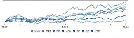
So, because of the risk in trading equities, it is vitally important to spread the risk amongst a large number of pairs.  That way, when one of your pairs trades inevitably blows up for one reason or another, the capital allocation is low enough not to cause irreparable damage to the overall portfolio.  Nor are you over-reliant on one or two star performers that may cease to contribute if, for example, one of the stock pairs is subject to a merger or takeover.

Does that mean that pairs trading is accessible only to managers with deep enough pockets to allocate broadly in the investment universe?  Yes and no.  On the one hand, of course, you need sufficient capital to allocate a meaningful sum to each of your pairs.  But pairs trading is highly efficient in its use of capital:  margin requirements are greatly reduced by the much lower risk of a dollar-neutral portfolio.  So your capital goes further than in would in a long-only strategy, for example.

How many pair combinations would you need to research to build an investment portfolio of the required size?  The answer might shock you:  millions.  Or  even tens of millions.  In the case of the Gemini Pairs strategy, for example, the universe comprises around 10m stock pairs and 200,000 ETF combinations.

It turns out to be much more challenging to find reliable stock pairs to trade than one might imagine, for reasons I am about to discuss.  So what tends to discourage investors from exploring pairs trading as an investment strategy is not because the strategy is inherently hard to understand; nor because the methods are unknown; nor because it requires vast amounts of investment capital to be viable.  It is that the research effort required to build a successful statistical arbitrage strategy is beyond the capability of the great majority of investors.

Before you become too discouraged, I will just say that there are at least two solutions to this challenge I can offer, which I will discuss later.

Methodology Isn’t a Decider

I have traded pairs successfully using all of the techniques described in the first part of the post (i.e. Ratio, Regression, Kalman and Copula methods).  Equally, I have seen a great many failed pairs strategies produced by using every available technique.  There is no silver bullet.  One often finds that a pair that perform poorly using the ratio method produces decent returns when a regression or Kalman Filter model is applied.  From experience, there is no pattern that allows you to discern which technique, if any, is gong to work.  You have to be prepared to try all of them, at least in back-test.

Correlation is Not the Answer

In a typical description of pairs trading the first order of business is often to look for a highly correlated pairs to trade.  While this makes sense as a starting point, it can never provide a complete answer.  The reason is well known:  correlations are unstable, and can often arise from random chance rather than as a result of a real connection between two stock processes.  The concept of spurious correlation is most easily grasped with an example, for instance:

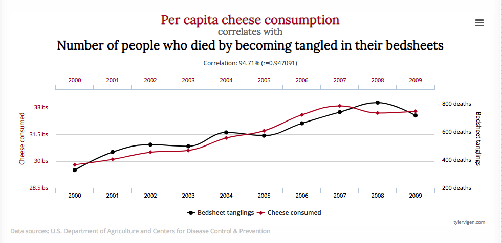
Of course, no rational person believes that there is a causal connection between cheese consumption and death by bedsheet entanglement – it is a spurious correlation that has arisen due to the random fluctuations in the two time series.  And because the correlation is spurious, the apparent relationship is likely to break down in future.

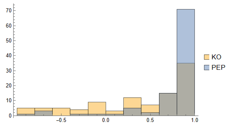
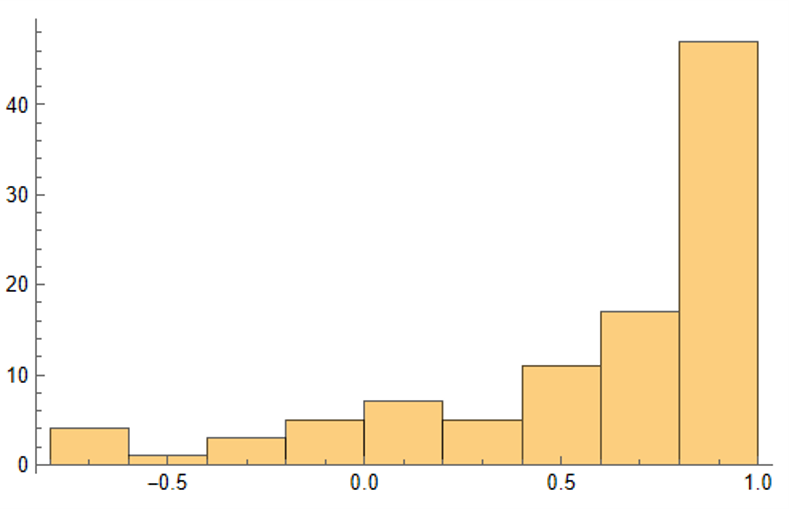
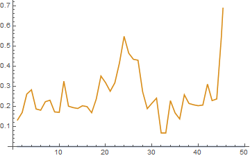
We can provide a slightly more realistic illustration as follows.  Let us suppose we have two correlated stocks, one with annual drift (i.e trend of 5% and annual volatility of 25%, the other with annual drift of 20% and annual volatility of 50%.  We assume that returns from the two processes follow a Normal distribution, with true correlation of 0.3.  Let’s assume that we sample the  returns for the two stocks over 90 days to estimate the correlation, simulating the real-world situation in which the true correlation is unknown.  Unlike in the real-world scenario, we can sample the 90-day returns many times (100,000 in this experiment) and look at the range of correlation estimates we observe:

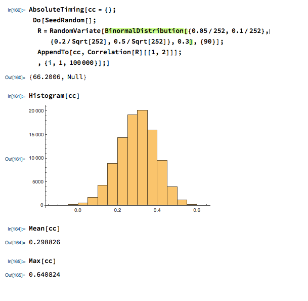
We find that, over the 100,000 repeated experiments the average correlation estimate is very close indeed to the true correlation.  However, in the real-world situation we only have a single observation, based on the returns from the two stock processes over the prior 90 days.  If we are very lucky, we might happen to pick a period in which the processes correlate at a level close to the true value of 0.3.  But as the experiment shows, we might be unlucky enough to see an estimate as high as 0.64, or as low as zero!

So when we look at historical data and use estimates of the correlation coefficient to gauge the strength of the relationship between two stocks, we are at the mercy of random variation in the sampling process, one that could suggest a much stronger (or weaker) connection than is actually the case.

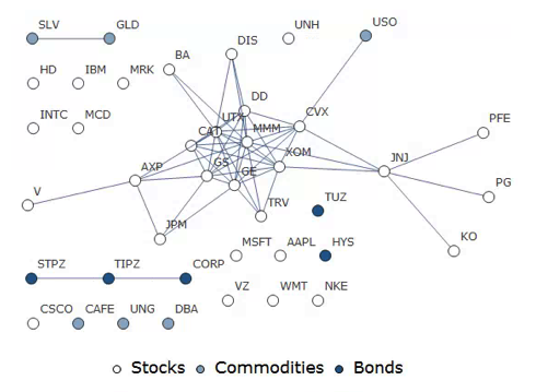
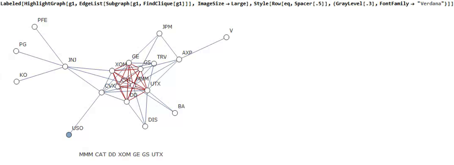
One is on firmer ground in selecting pairs of stocks in the same sector, for example oil or gold-mining stocks, because we are able to identify causal factors that should provide a basis for a reliable correlation, such as the price of oil or gold.  This is indeed one of the “screens” that statistical arbitrageurs often use to select pairs for analysis.  But there are many examples of stocks that “ought” to be correlated but which nonetheless break down and drift apart.  This can happen for many reasons:  changes in the capital structure of one of the companies; a major product launch;  regulatory action; or corporate actions such as mergers and takeovers.

The bottom line is that correlation, while important, is not by itself a sufficiently reliable measure to provide a basis for pair selection.

Cointegration: the Drunk and His Dog

Suppose you see two drunks (i.e., two random walks) wandering around. The drunks don’t know each other (they’re independent), so there’s no meaningful relationship between their paths.

But suppose instead you have a drunk walking with his dog. This time there is a connection. What’s the nature of this connection? Notice that although each path individually is still an unpredictable random walk, given the location of one of the drunk or dog, we have a pretty good idea of where the other is; that is, the distance between the two is fairly predictable. (For example, if the dog wanders too far away from his owner, he’ll tend to move in his direction to avoid losing him, so the two stay close together despite a tendency to wander around on their own.) We describe this relationship by saying that the drunk and her dog form a cointegrating pair.

In more technical terms, if we have two non-stationary time series X and Y that become stationary when differenced (these are called integrated of order one series, or I(1) series; random walks are one example) such that some linear combination of X and Y is stationary (aka, I(0)), then we say that X and Y are cointegrated. In other words, while neither X nor Y alone hovers around a constant value, some combination of them does, so we can think of cointegration as describing a particular kind of long-run equilibrium relationship. (The definition of cointegration can be extended to multiple time series, with higher orders of integration.)

Other examples of cointegrated pairs:

  • Income and consumption: as income increases/decreases, so too does consumption.
  • Size of police force and amount of criminal activity
  • A book and its movie adaptation: while the book and the movie may differ in small details, the overall plot will remain the same.
  • Number of patients entering or leaving a hospital

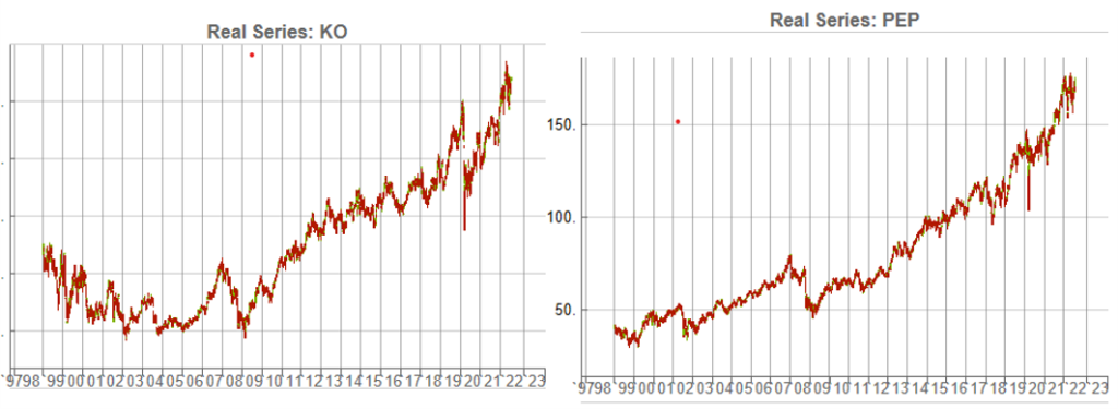
So why do we care about cointegration? Someone else can probably give more econometric applications, but in quantitative finance, cointegration forms the basis of the pairs trading strategy: suppose we have two cointegrated stocks X and Y, with the particular (for concreteness) cointegrating relationship X – 2Y = Z, where Z is a stationary series of zero mean. For example, X could be McDonald’s, Y could be Burger King, and the cointegration relationship would mean that X tends to be priced twice as high as Y, so that when X is more than twice the price of Y, we expect X to move down or Y to move up in the near future (and analogously, if X is less than twice the price of Y, we expect X to move up or Y to move down). This suggests the following trading strategy: if X – 2Y > d, for some positive threshold d, then we should sell X and buy Y (since we expect X to decrease in price and Y to increase), and similarly, if X – 2Y < -d, then we should buy X and sell Y.

So how do you detect cointegration? There are several different methods, but the simplest is probably the Engle-Granger test, which works roughly as follows:

  • Check that Xt and Yt are both I(1).
  • Estimate the cointegrating relationship =+Yt=aXt+et by ordinary least squares.
  • Check that the cointegrating residuals et are stationary (say, by using a so-called unit root test, e.g., the Dickey-Fuller test).

Also, something else that should perhaps be mentioned is the relationship between cointegration and error-correction mechanisms: suppose we have two cointegrated series ,Xt,Yt, with autoregressive representations

=1+1+Xt=aXt−1+bYt−1+ut
=1+1+Yt=cXt−1+dYt−1+vt

By the Granger representation theorem (which is actually a bit more general than this), we then have

Δ=1(11)+ΔXt=α1(Yt−1−βXt−1)+ut
Δ=2(11)+ΔYt=α2(Yt−1−βXt−1)+vt

where 11(0)Yt−1−βXt−1∼I(0) is the cointegrating relationship. Regarding 11Yt−1−βXt−1 as the extent of disequilibrium from the long-run relationship, and the αi as the speed (and direction) at which the time series correct themselves from this disequilibrium, we can see that this formalizes the way cointegrated variables adjust to match their long-run equilibrium.

So, just to summarize a bit, cointegration is an equilibrium relationship between time series that individually aren’t in equilibrium (you can kind of contrast this with (Pearson) correlation, which describes a linear relationship), and it’s useful because it allows us to incorporate both short-term dynamics (deviations from equilibrium) and long-run expectations , i.e. corrections to equilibrium.  (My thanks to Edwin Chen for this entertaining explanation)

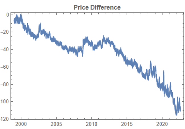
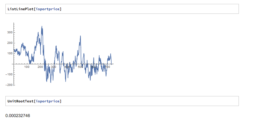
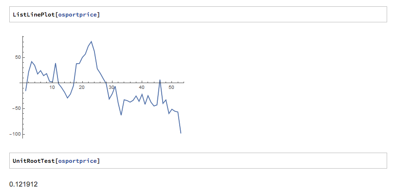
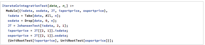
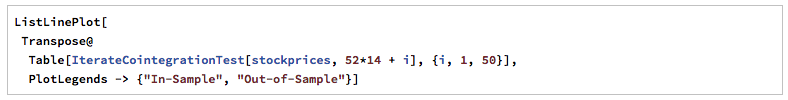
Cointegration is Not the Answer

So a typical workflow for researching possible pairs trade might be to examine a large number of pairs in a sector of interest, select those that meet some correlation threshold (e.e. 90%), test those pairs for cointegration and select those that appear to be cointegrated.  The problem is:  it doesn’t work!  The pairs thrown up by this process are likely to work for a while, but many (even the majority) will break down at some point, typically soon after you begin live trading.  `The reason is that all of the major statistical tests for cointegration have relatively low power and pairs that are apparently cointegrated break down suddenly, with consequential losses for the trader.  The following posts delves into the subject in some detail:


Other Practical “Gotchas”

Apart from correlations/cointegration breakdowns there is a long list of things that can go wrong with a pairs trade that the practitioner needs to take account of, for instance:

  • A stock may become difficult or expensive to short
  • The overall backtest performance stats for a pair may look great, but the P&L per share is too small to overcome trading costs and other frictions.
  • Corporate actions (mergers, takeovers) and earnings can blow up one side of an otherwise profitable pair.
  • It is possible to trade passively, crossing the spread  to trade the other leg when the first leg trades.  But this trade expression is challenging to test.  If paying the spread on both legs is going to jeopardize the profitability of the strategy, it is probably better to reject the pair.
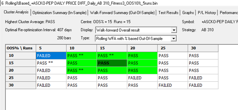
What Works

From my experience, the testing phase of the process of building a statistical arbitrage strategy is absolutely critical.  By this I mean that, after screening for correlation and cointegration, and back-testing all of the possible types of model, it is essential to conduct an extensive simulation test over a period of several weeks before adding a new pair to the production system.  Testing is important for any algorithmic strategy, of course, but it is an integral part of the selection process where pairs trading is concerned.  You should expect 60% to 80% of your candidates to fail in simulated trading, even after they have been carefully selected and thoroughly back-tested.  The good good news is that those pairs that pass the final stage of testing usually are successful in a production setting.

Implementation

Putting all of this information together, it should be apparent that the major challenge in pairs trading lies not so much in understanding and implementing methodologies and techniques, but in implementing the research process on an industrial scale, sufficient to collate and analyze tens of millions of pairs. This is beyond the reach of most retail investors, and indeed, many small trading firms:  I once worked with a trading firm for over a year on a similar research project, but in the end it proved to be capabilities of even their highly competent development team.

So does this mean that for the average quantitative strategist investors statistical arbitrage must remain an investment concept of purely theoretical interest?  Actually, no.  Firstly, for the investor, there are plenty of investment products available that they can access via hedge fund structures (or even our algotrading platform, as I have previously mentioned).

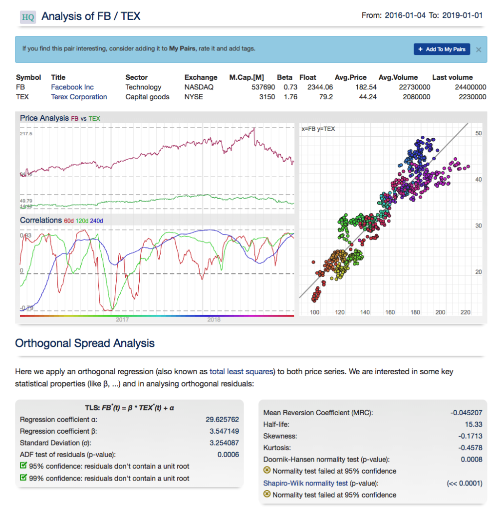
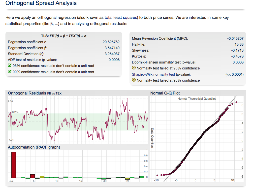
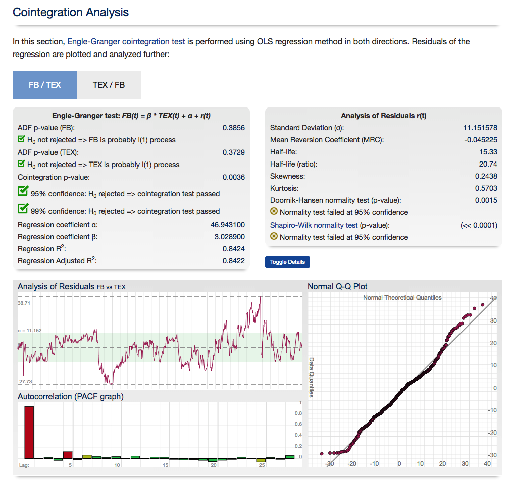
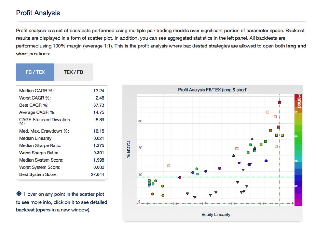
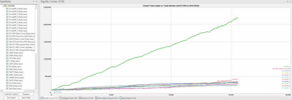
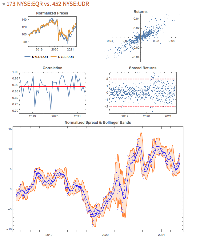
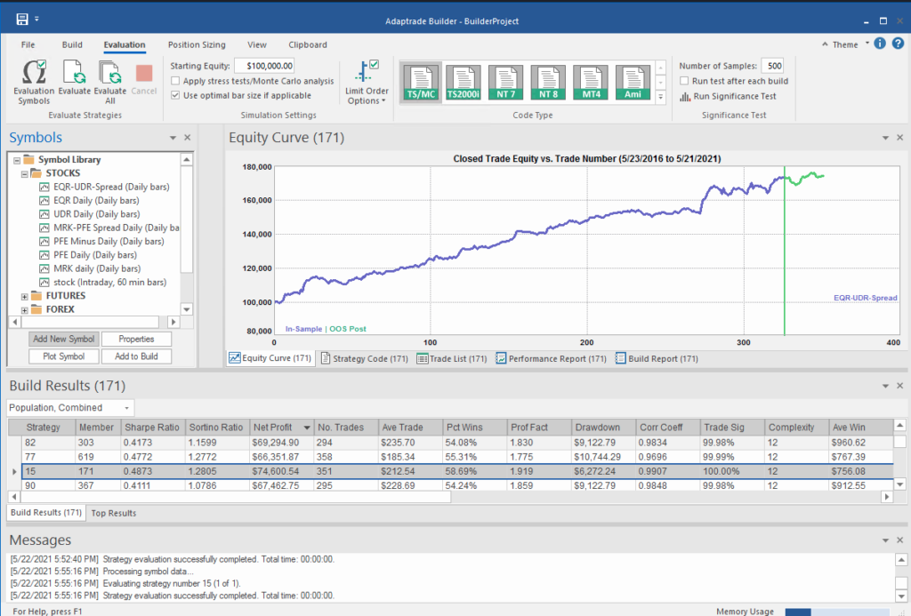
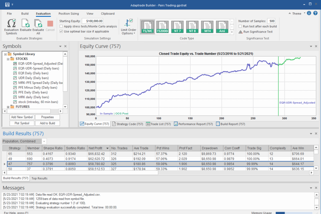
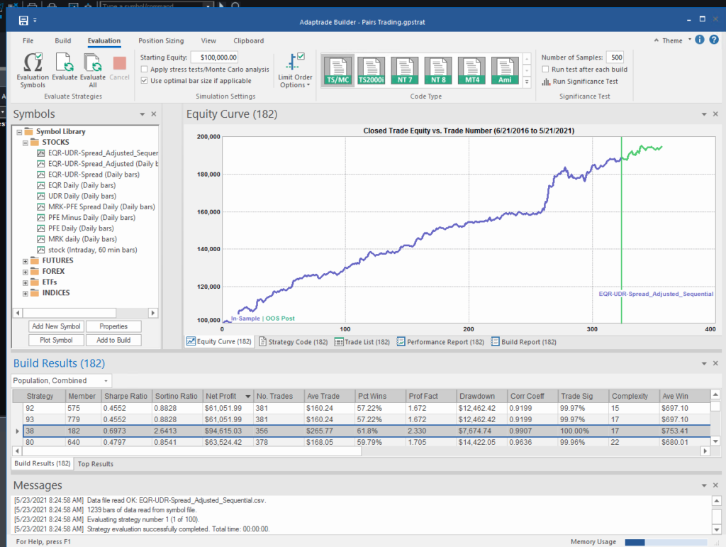
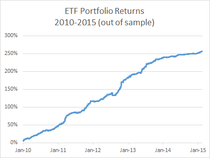
For those interested in building stat arb strategies there is an excellent resource that collates all of the data and analysis on tens of millions of stock pairs that enables the researcher to identify promising pairs, test their level of cointegration, backtest strategies using different methodologies and even put selected pars strategies into production (see example below).

Those interested should contact me for more information.


Developing Long/Short ETF Strategies

Recently I have been working on the problem of how to construct large portfolios of cointegrated securities.  My focus has been on ETFs rather that stocks, although in principle the methodology applies equally well to either, of course.

My preference for ETFs is due primarily to the fact that  it is easier to achieve a wide diversification in the portfolio with a more limited number of securities: trading just a handful of ETFs one can easily gain exposure, not only to the US equity market, but also international equity markets, currencies, real estate, metals and commodities. Survivorship bias, shorting restrictions  and security-specific risk are also less of an issue with ETFs than with stocks (although these problems are not too difficult to handle).

On the downside, with few exceptions ETFs tend to have much shorter histories than equities or commodities.  One also has to pay close attention to the issue of liquidity. That said, I managed to assemble a universe of 85 ETF products with histories from 2006 that have sufficient liquidity collectively to easily absorb an investment of several hundreds of  millions of dollars, at minimum.

The Cardinality Problem

The basic methodology for constructing a long/short portfolio using cointegration is covered in an earlier post.   But problems arise when trying to extend the universe of underlying securities.  There are two challenges that need to be overcome.

Magic Cube.112

The first issue is that, other than the simple regression approach, more advanced techniques such as the Johansen test are unable to handle data sets comprising more than about a dozen securities. The second issue is that the number of possible combinations of cointegrated securities quickly becomes unmanageable as the size of the universe grows.  In this case, even taking a subset of just six securities from the ETF universe gives rise to a total of over 437 million possible combinations (85! / (79! * 6!).  An exhaustive test of all the possible combinations of a larger portfolio of, say, 20 ETFs, would entail examining around 1.4E+19 possibilities.

Given the scale of the computational problem, how to proceed? One approach to addressing the cardinality issue is sparse canonical correlation analysis, as described in Identifying Small Mean Reverting Portfolios,  d’Aspremont (2008). The essence of the idea is something like this. Suppose you find that, in a smaller, computable universe consisting of just two securities, a portfolio comprising, say, SPY and QQQ was  found to be cointegrated.  Then, when extending consideration to portfolios of three securities, instead of examining every possible combination, you might instead restrict your search to only those portfolios which contain SPY and QQQ. Having fixed the first two selections, you are left with only 83 possible combinations of three securities to consider.  This process is repeated as you move from portfolios comprising 3 securities to 4, 5, 6, … etc.

Other approaches to the cardinality problem are  possible.  In their 2014 paper Sparse, mean reverting portfolio selection using simulated annealing,  the Hungarian researchers Norbert Fogarasi and Janos Levendovszky consider a new optimization approach based on simulated annealing.  I have developed my own, hybrid approach to portfolio construction that makes use of similar analytical methodologies. Does it work?

A Cointegrated Long/Short ETF Basket

Below are summarized the out-of-sample results for a portfolio comprising 21 cointegrated ETFs over the period from 2010 to 2015.  The basket has broad exposure (long and short) to US and international equities, real estate, currencies and interest rates, as well as exposure in banking, oil and gas and other  specific sectors.

The portfolio was constructed using daily data from 2006 – 2009, and cointegration vectors were re-computed annually using data up to the end of the prior year.  I followed my usual practice of using daily data comprising “closing” prices around 12pm, i.e. in the middle of the trading session, in preference to prices at the 4pm market close.  Although liquidity at that time is often lower than at the close, volatility also tends to be muted and one has a period of perhaps as much at two hours to try to achieve the arrival price. I find this to be a more reliable assumption that the usual alternative.

Fig 2   Fig 1 The risk-adjusted performance of the strategy is consistently outstanding throughout the out-of-sample period from 2010.  After a slowdown in 2014, strategy performance in the first quarter of 2015 has again accelerated to the level achieved in earlier years (i.e. with a Sharpe ratio above 4).

Another useful test procedure is to compare the strategy performance with that of a portfolio constructed using standard mean-variance optimization (using the same ETF universe, of course).  The test indicates that a portfolio constructed using the traditional Markowitz approach produces a similar annual return, but with 2.5x the annual volatility (i.e. a Sharpe ratio of only 1.6).  What is impressive about this result is that the comparison one is making is between the out-of-sample performance of the strategy vs. the in-sample performance of a portfolio constructed using all of the available data.

Having demonstrated the validity of the methodology,  at least to my own satisfaction, the next step is to deploy the strategy and test it in a live environment.  This is now under way, using execution algos that are designed to minimize the implementation shortfall (i.e to minimize any difference between the theoretical and live performance of the strategy).  So far the implementation appears to be working very well.

Once a track record has been built and audited, the really hard work begins:  raising investment capital!

Cointegration Breakdown

The Low Power of Cointegration Tests

One of the perennial difficulties in developing statistical arbitrage strategies is the lack of reliable methods of estimating a stationary portfolio comprising two or more securities. In a prior post (below) I discussed at some length one of the primary reasons for this, i.e. the lower power of cointegration tests. In this post I want to explore the issue in more depth, looking at the standard Johansen test Procedure to estimate cointegrating vectors.

Johansen Test for Cointegration

Start with some weekly data for an ETF triplet analyzed in Ernie Chan’s book:

After downloading the weekly close prices for the three ETFs we divide the data into 14 years of in-sample data and 1 year out of sample:

We next apply the Johansen test, using code kindly provided by Amanda Gerrish:

We find evidence of up to three cointegrating vectors at the 95% confidence level:


Let’s take a look at the vector coefficients (laid out in rows, in Amanda’s function):

In-Sample vs. Out-of-Sample testing

We now calculate the in-sample and out-of-sample portfolio values using the first cointegrating vector:

The portfolio does indeed appear to be stationary, in-sample, and this is confirmed by the unit root test, which rejects the null hypothesis of a unit root:

Unfortunately (and this is typically the case) the same is not true for the out of sample period:

More Data Doesn’t Help

The problem with the nonstationarity of the out-of-sample estimated portfolio values is not mitigated by adding more in-sample data points and re-estimating the cointegrating vector(s):

We continue to add more in-sample data points, reducing the size of the out-of-sample dataset correspondingly. But none of the tests for any of the out-of-sample datasets is able to reject the null hypothesis of a unit root in the portfolio price process:


The Challenge of Cointegration Testing in Real Time

In our toy problem we know the out-of-sample prices of the constituent ETFs, and can therefore test the stationarity of the portfolio process out of sample. In a real world application, that discovery could only be made in real time, when the unknown, future ETFs prices are formed. In that scenario, all the researcher has to go on are the results of in-sample cointegration analysis, which demonstrate that the first cointegrating vector consistently yields a portfolio price process that is very likely stationary in sample (with high probability).

The researcher might understandably be persuaded, wrongly, that the same is likely to hold true in future. Only when the assumed cointegration relationship falls apart in real time will the researcher then discover that it’s not true, incurring significant losses in the process, assuming the research has been translated into some kind of trading strategy.

A great many analysts have been down exactly this path, learning this important lesson the hard way. Nor do additional “safety checks” such as, for example, also requiring high levels of correlation between the constituent processes add much value. They might offer the researcher comfort that a “belt and braces” approach is more likely to succeed, but in my experience it is not the case: the problem of non-stationarity in the out of sample price process persists.

Conclusion:  Why Cointegration Breaks Down

We have seen how a portfolio of ETFs consistently estimated to be cointegrated in-sample, turns out to be non-stationary when tested out-of-sample.  This goes to the issue of the low power of cointegration test, and their inability to estimate cointegrating vectors with sufficient accuracy.  Analysts relying on standard tests such as the Johansen procedure to design their statistical arbitrage strategies are likely to be disappointed by the regularity with which their strategies break down in live trading.