Genetic Programming Archives - QUANTITATIVE RESEARCH AND TRADING

May 23, 2021May 25, 2021

Machine Learning Based Statistical Arbitrage

I have written extensively about statistical arbitrage strategies in previous posts, for example:

Successful Statistical Arbitrage

Developing Statistical Arbitrage Strategies Using Cointegration

Pairs Trading with Copulas

Applying Machine Learning in Statistical Arbitrage

In this series of posts I want to focus on applications of machine learning in stat arb and pairs trading, including genetic algorithms, deep neural networks and reinforcement learning.

Pair Selection

Let’s begin with the subject of pairs selection, to set the scene. The way this is typically handled is by looking at historical correlations and cointegration in a large universe of pairs. But there are serious issues with this approach, as described in this post:

Cointegration Breakdown

Instead I use a metric that I call the correlation signal, which I find to be a more reliable indicator of co-movement in the underlying asset processes. I wont delve into the details here, but you can get the gist from the following:

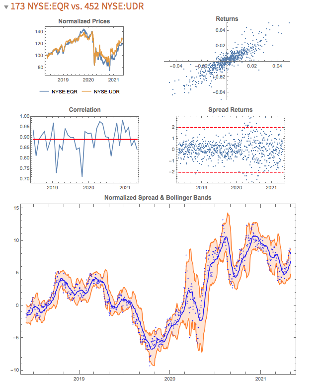
The search algorithm considers pairs in the S&P 500 membership and ranks them in descending order of correlation information. Pairs with the highest values (typically of the order of 100, or greater) tend to be variants of the same underlying stock, such as GOOG vs GOOGL, which is an indication that the metric “works” (albeit that such pairs offer few opportunities at low frequency). The pair we are considering here has a correlation signal value of around 14, which is also very high indeed.

Trading Strategy Development

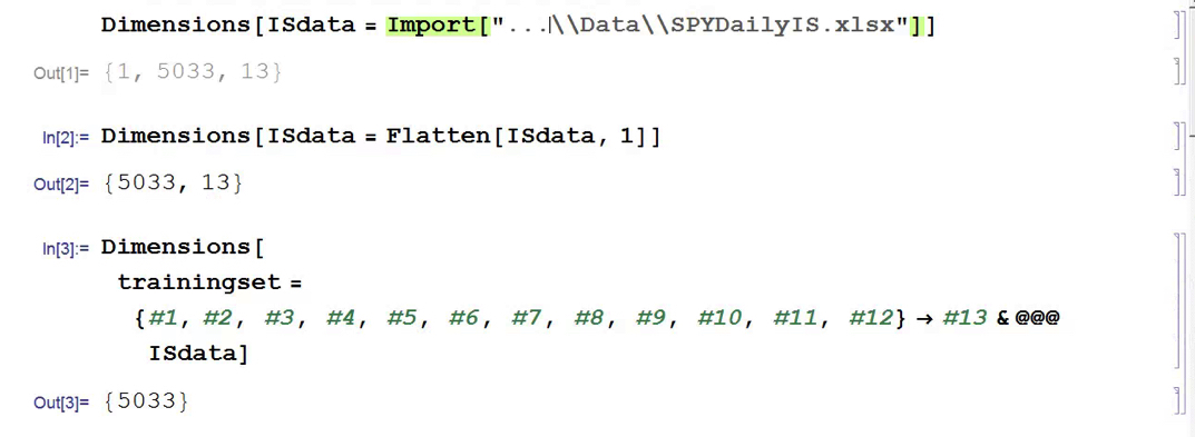
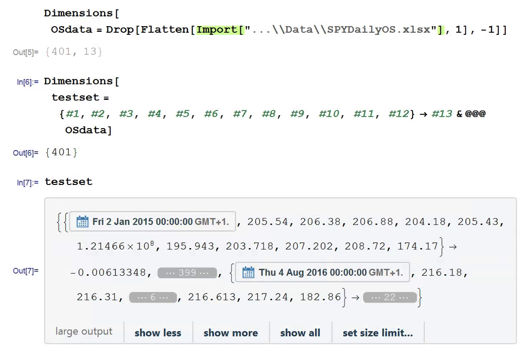
We begin by collecting five years of returns series for the two stocks:

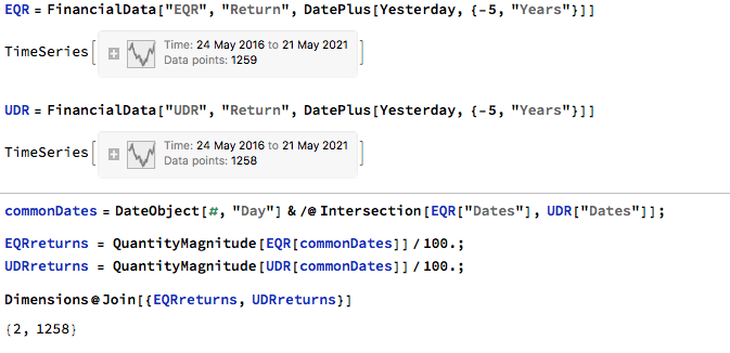
The first approach we’ll consider is the unadjusted spread, being the difference in returns between the two series, from which we crate a normalized spread “price”, as follows.

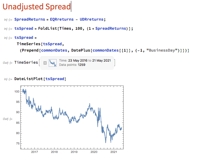
This methodology is frowned upon as the resultant spread is unlikely to be stationary, as you can see for this example in the above chart. But it does have one major advantage in terms of implementation: the same dollar value is invested in both long and short legs of the spread, making it the most efficient approach in terms of margin utilization and capital cost – other approaches entail incurring an imbalance in the dollar value of the two legs.

But back to nonstationarity. The problem is that our spread price series looks like any other asset price process – it trends over long periods and tends to wander arbitrarily far from its starting point. This is NOT the outcome that most statistical arbitrageurs are looking to achieve. On the contrary, what they want to see is a stationary process that will tend to revert to its mean value whenever it moves too far in one direction.

Still, this doesn’t necessarily determine that this approach is without merit. Indeed, it is a very typical trading strategy amongst futures traders for example, who are often looking for just such behavior in their trend-following strategies. Their argument would be that futures spreads (which are often constructed like this) exhibit clearer, longer lasting and more durable trends than in the underlying futures contracts, with lower volatility and market risk, due to the offsetting positions in the two legs. The argument has merit, no doubt. That said, spreads of this kind can nonetheless be extremely volatile.

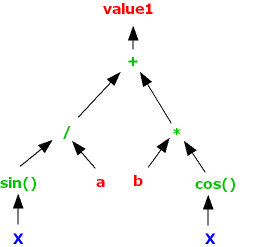
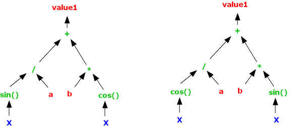
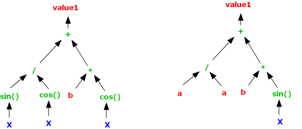
So how do we trade such a spread? One idea is to add machine learning into the mix and build trading systems that will seek to capitalize on long term trends. We can do that in several ways, one of which is to apply genetic programming techniques to generate potential strategies that we can backtest and evaluate. For more detail on the methodology, see:

A Primer on Genetic Programming

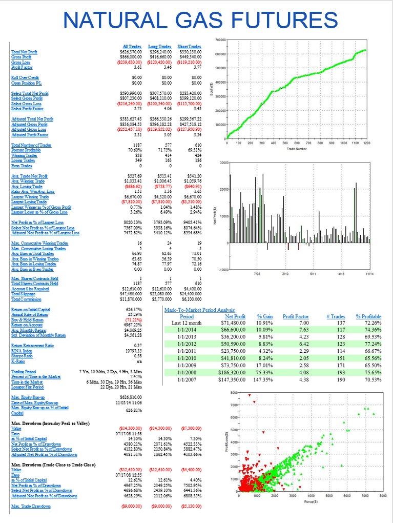
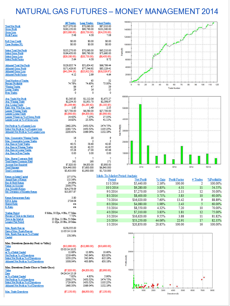
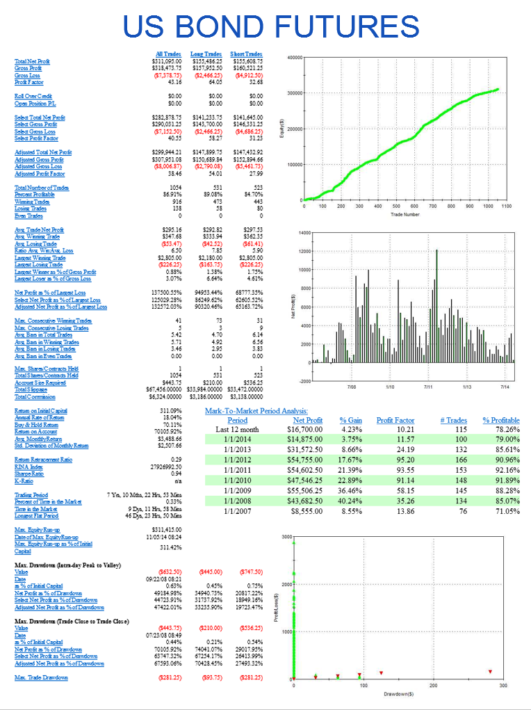
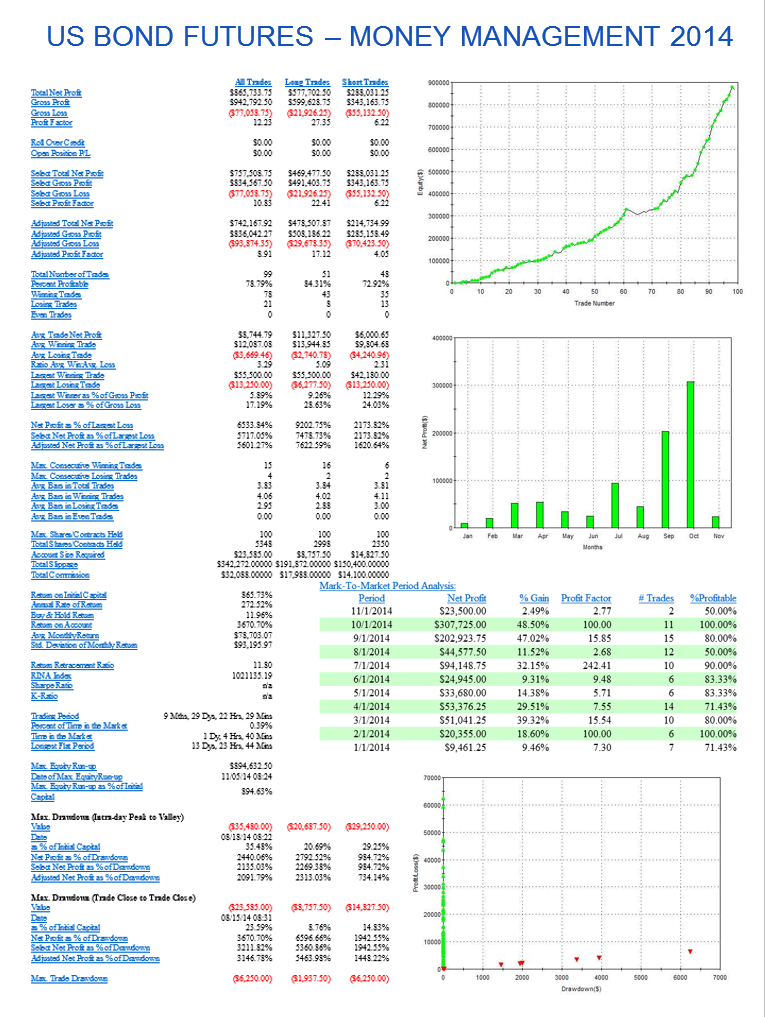
I built an entire hedge fund using this approach in the early 2000’s (when machine learning was entirely unknown to the general investing public). These days there are some excellent software applications for generating trading systems and I particularly like Mike Bryant’s Adaptrade Builder, which was used to create the strategies shown below:

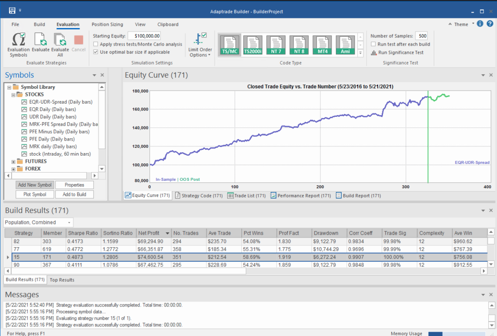
Builder has no difficulty finding strategies that produce a smooth equity curve, with decent returns, low drawdowns and acceptable Sharpe Ratios and Profit Factors – at least in backtest! Of course, there is a way to go here in terms of evaluating such strategies and proving their robustness. But it’s an excellent starting point for further R&D.

But let’s move on to consider the “standard model” for pairs trading. The way this works is that we consider a linear model of the form

Y(t) = beta * X(t) + e(t)

Where Y(t) is the returns series for stock 1, X(t) is the returns series in stock 2, e(t) is a stationary random error process and beta (is this model) is a constant that expresses the linear relationship between the two asset processes. The idea is that we can form a spread process that is stationary:

Y(t) – beta * X(t) = e(t)

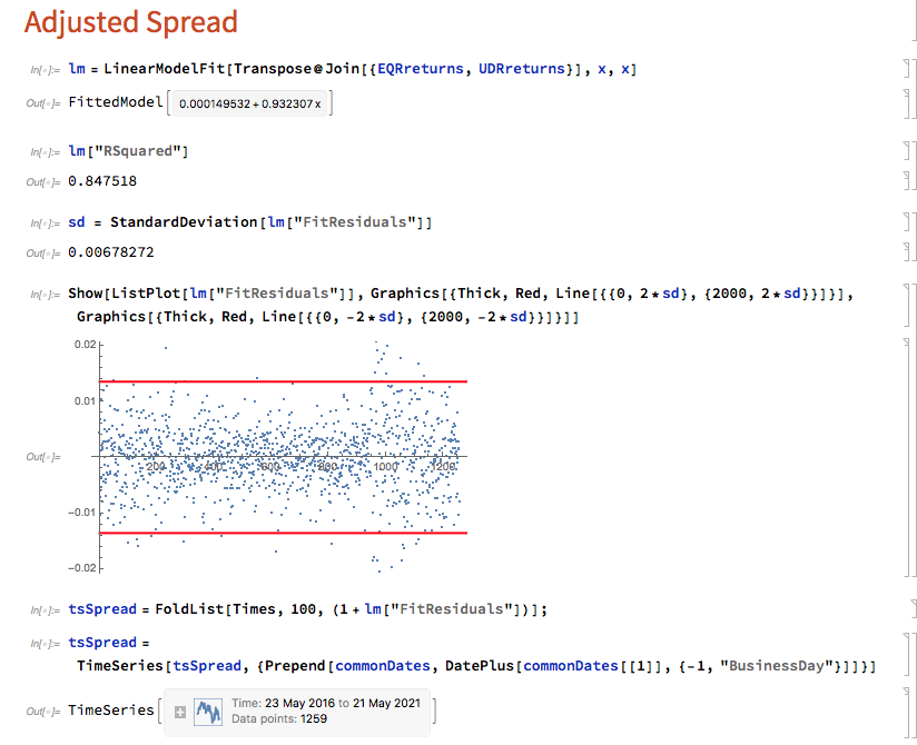
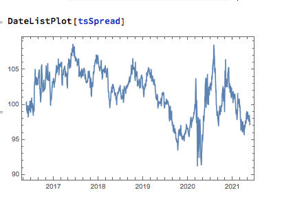
In this case we estimate beta by linear regression to be 0.93. The residual spread process has a mean very close to zero, and the spread price process remains within a range, which means that we can buy it when it gets too low, or sell it when it becomes too high, in the expectation that it will revert to the mean:

In this approach, “buying the spread” means purchasing shares to the value of, say, $1M in stock 1, and selling beta * $1M of stock 2 (around $930,000). While there is a net dollar imbalance in the dollar value of the two legs, the margin impact tends to be very small indeed, while the overall portfolio is much more stable, as we have seen.

The classical procedure is to buy the spread when the spread return falls 2 standard deviations below zero, and sell the spread when it exceeds 2 standard deviations to the upside. But that leaves a lot of unanswered questions, such as:

After you buy the spread, when should you sell it?
Should you use a profit target?
Where should you set a stop-loss?
Do you increase your position when you get repeated signals to go long (or short)?
Should you use a single, or multiple entry/exit levels?

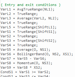
And so on – there are a lot of strategy components to consider. Once again, we’ll let genetic programming do the heavy lifting for us:

What’s interesting here is that the strategy selected by the Builder application makes use of the Bollinger Band indicator, one of the most common tools used for trading spreads, especially when stationary (although note that it prefers to use the Opening price, rather than the usual close price):

Ok so far, but in fact I cheated! I used the entire data series to estimate the beta coefficient, which is effectively feeding forward-information into our model. In reality, the data comes at us one day at a time and we are required to re-estimate the beta every day.

Let’s approximate the real-life situation by re-estimating beta, one day at a time. I am using an expanding window to do this (i.e. using the entire data series up to each day t), but is also common to use a fixed window size to give a “rolling” estimate of beta in which the latest data plays a more prominent part in the estimation. The process now looks like this:

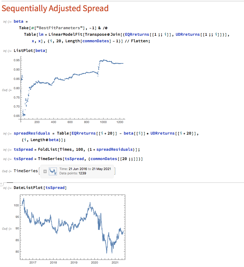
Here we use OLS to produce a revised estimate of beta on each trading day. So our model now becomes:

Y(t) = beta(t) * X(t) + e(t)

i.e. beta is now time-varying, as can be seen from the chart above.

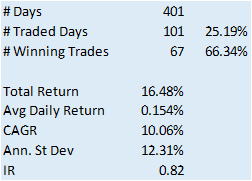
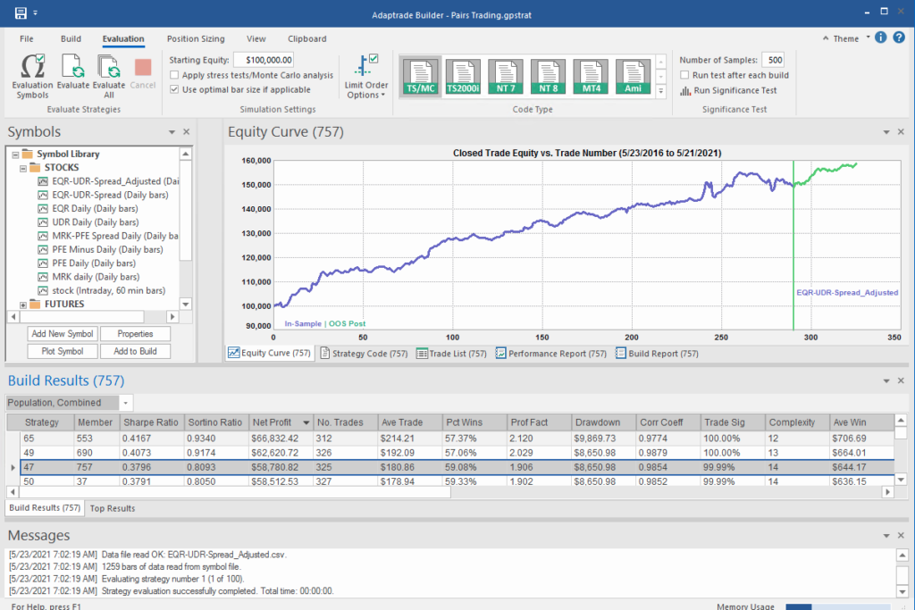
The synthetic spread price appears to be stationary (we can test this), although perhaps not to the same degree as in the previous example, where we used the entire data series to estimate a single, constant beta. So we might anticipate that out ML algorithm would experience greater difficulty producing attractive trading models. But, not a bit of it – it turns out that we are able to produce systems that are just as high performing as before:

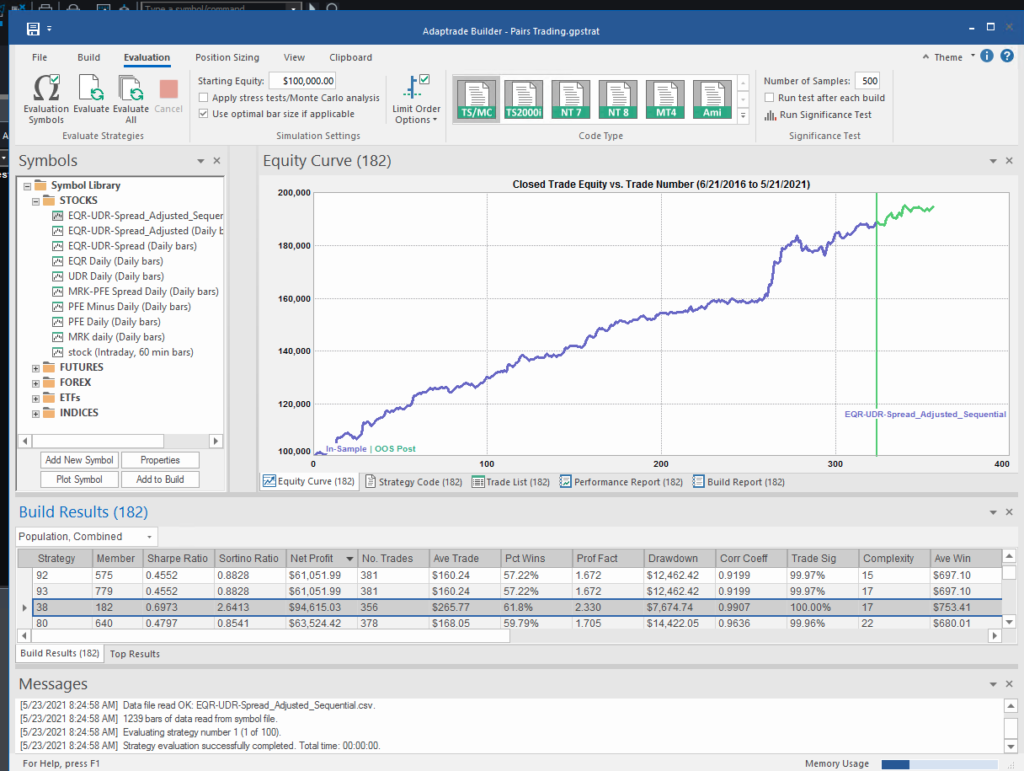
In fact this strategy has higher returns, Sharpe Ratio, Sortino Ratio and lower drawdown than many of the earlier models.

Conclusion

The purpose of this post was to show how we can combine the standard approach to statistical arbitrage, which is based on classical econometric theory, with modern machine learning algorithms, such as genetic programming. This frees us to consider a very much wider range of possible trade entry and exit strategies, beyond the rather simplistic approach adopted when pairs trading was first developed. We can deploy multiple trade entry levels and stop loss levels to manage risk, dynamically size the trade according to current market conditions and give emphasis to alternative performance characteristics such as maximum drawdown, or Sharpe or Sortino ratio, in addition to strategy profitability.

The programatic nature of the strategies developed in the way also make them very amenable to optimization, Monte Carlo simulation and stress testing.

This is but one way of adding machine learning methodologies to the mix. In a series of follow-up posts I will be looking at the role that other machine learning techniques – such as deep learning and reinforcement learning – can play in improving the performance characteristics of the classical statistical arbitrage strategy.

November 19, 2019

Strategy Portfolio Construction

August 27, 2019

Machine Learning Trading Systems

The SPDR S&P 500 ETF (SPY) is one of the widely traded ETF products on the market, with around $200Bn in assets and average turnover of just under 200M shares daily. So the likelihood of being able to develop a money-making trading system using publicly available information might appear to be slim-to-none. So, to give ourselves a fighting chance, we will focus on an attempt to predict the overnight movement in SPY, using data from the prior day’s session.

In addition to the open/high/low and close prices of the preceding day session, we have selected a number of other plausible variables to build out the feature vector we are going to use in our machine learning model:

The daily volume
The previous day’s closing price
The 200-day, 50-day and 10-day moving averages of the closing price
The 252-day high and low prices of the SPY series

We will attempt to build a model that forecasts the overnight return in the ETF, i.e. [O(t+1)-C(t)] / C(t)

In this exercise we use daily data from the beginning of the SPY series up until the end of 2014 to build the model, which we will then test on out-of-sample data running from Jan 2015-Aug 2016. In a high frequency context a considerable amount of time would be spent evaluating, cleaning and normalizing the data. Here we face far fewer problems of that kind. Typically one would standardized the input data to equalize the influence of variables that may be measured on scales of very different orders of magnitude. But in this example all of the input variables, with the exception of volume, are measured on the same scale and so standardization is arguably unnecessary.

First, the in-sample data is loaded and used to create a training set of rules that map the feature vector to the variable of interest, the overnight return:

In Mathematica 10 Wolfram introduced a suite of machine learning algorithms that include regression, nearest neighbor, neural networks and random forests, together with functionality to evaluate and select the best performing machine learning technique. These facilities make it very straightfoward to create a classifier or prediction model using machine learning algorithms, such as this handwriting recognition example:

We create a predictive model on the SPY trainingset, allowing Mathematica to pick the best machine learning algorithm:

There are a number of options for the Predict function that can be used to control the feature selection, algorithm type, performance type and goal, rather than simply accepting the defaults, as we have done here:

Having built our machine learning model, we load the out-of-sample data from Jan 2015 to Aug 2016, and create a test set:

We next create a PredictionMeasurement object, using the Nearest Neighbor model , that can be used for further analysis:

There isn’t much dispersion in the model forecasts, which all have positive value. A common technique in such cases is to subtract the mean from each of the forecasts (and we may also standardize them by dividing by the standard deviation).

The scatterplot of actual vs. forecast overnight returns in SPY now looks like this:

There’s still an obvious lack of dispersion in the forecast values, compared to the actual overnight returns, which we could rectify by standardization. In any event, there appears to be a small, nonlinear relationship between forecast and actual values, which holds out some hope that the model may yet prove useful.

From Forecasting to Trading

There are various methods of deploying a forecasting model in the context of creating a trading system. The simplest route, which we will take here, is to apply a threshold gate and convert the filtered forecasts directly into a trading signal. But other approaches are possible, for example:

Combining the forecasts from multiple models to create a prediction ensemble
Using the forecasts as inputs to a genetic programming model
Feeding the forecasts into the input layer of a neural network model designed specifically to generate trading signals, rather than forecasts

In this example we will create a trading model by applying a simple filter to the forecasts, picking out only those values that exceed a specified threshold. This is a standard trick used to isolate the signal in the model from the background noise. We will accept only the positive signals that exceed the threshold level, creating a long-only trading system. i.e. we ignore forecasts that fall below the threshold level. We buy SPY at the close when the forecast exceeds the threshold and exit any long position at the next day’s open. This strategy produces the following pro-forma results:

Conclusion

The system has some quite attractive features, including a win rate of over 66% and a CAGR of over 10% for the out-of-sample period.

Obviously, this is a very basic illustration: we would want to factor in trading commissions, and the slippage incurred entering and exiting positions in the post- and pre-market periods, which will negatively impact performance, of course. On the other hand, we have barely begun to scratch the surface in terms of the variables that could be considered for inclusion in the feature vector, and which may increase the explanatory power of the model.

In other words, in reality, this is only the beginning of a lengthy and arduous research process. Nonetheless, this simple example should be enough to give the reader a taste of what’s involved in building a predictive trading model using machine learning algorithms.

September 21, 2018

Building Systematic Strategies – A New Approach

Anyone active in the quantitative space will tell you that it has become a great deal more competitive in recent years. Many quantitative trades and strategies are a lot more crowded than they used to be and returns from existing strategies are on the decline.

THE CHALLENGE

Meanwhile, costs have been steadily rising, as the technology arms race has accelerated, with more money being spent on hardware, communications and software than ever before. As lead times to develop new strategies have risen, the cost of acquiring and maintaining expensive development resources have spiraled upwards. It is getting harder to find new, profitable strategies, due in part to the over-grazing of existing methodologies and data sets (like the E-Mini futures, for example). There has, too, been a change in the direction of quantitative research in recent years. Where once it was simply a matter of acquiring the fastest pipe to as many relevant locations as possible, the marginal benefit of each extra $ spent on infrastructure has since fallen rapidly. New strategy research and development is now more model-driven than technology driven.

THE OPPORTUNITY

What is needed at this point is a new approach: one that accelerates the process of identifying new alpha signals, prototyping and testing new strategies and bringing them into production, leveraging existing battle-tested technologies and trading platforms.

GENETIC PROGRAMMING

Genetic programming, which has been around since the 1990’s when its use was pioneered in proteomics, enjoys significant advantages over traditional research and development methodologies.

GP is an evolutionary-based algorithmic methodology in which a system is given a set of simple rules, some data, and a fitness function that produces desired outcomes from combining the rules and applying them to the data. The idea is that, by testing large numbers of possible combinations of rules, typically in the millions, and allowing the most successful rules to propagate, eventually we will arrive at a strategy solution that offers the required characteristics.

ADVANTAGES OF GENETIC PROGRAMMING

The potential benefits of the GP approach are considerable: not only are strategies developed much more quickly and cost effectively (the price of some software and a single CPU vs. a small army of developers), the process is much more flexible. The inflexibility of the traditional approach to R&D is one of its principle shortcomings. The researcher produces a piece of research that is subsequently passed on to the development team. Developers are usually extremely rigid in their approach: when asked to deliver X, they will deliver X, not some variation on X. Unfortunately research is not an exact science: what looks good in a back-test environment may not pass muster when implemented in live trading. So researchers need to “iterate around” the idea, trying different combinations of entry and exit logic, for example, until they find a variant that works. Developers are lousy at this; GP systems excel at it.

CHALLENGES FOR THE GENETIC PROGRAMMING APPROACH

So enticing are the potential benefits of GP that it begs the question as to why the approach hasn’t been adopted more widely. One reason is the strong preference amongst researchers for an understandable – and testable – investment thesis. Researchers – and, more importantly, investors – are much more comfortable if they can articulate the premise behind a strategy. Even if a trade turns out to be a loser, we are generally more comfortable buying a stock on the supposition of, say, a positive outcome of a pending drug trial, than we are if required to trust the judgment of a black box, whose criteria are inherently unobservable.

Added to this, the GP approach suffers from three key drawbacks: data sufficiency, data mining and over-fitting. These are so well known that they hardly require further rehearsal. There have been many adverse outcomes resulting from poorly designed mechanical systems curve fitted to the data. Anyone who was active in the space in the 1990s will recall the hype over neural networks and the over-exaggerated claims made for their efficacy in trading system design. Genetic Programming, a far more general and powerful concept, suffered unfairly from the ensuing adverse publicity, although it does face many of the same challenges.

A NEW APPROACH

I began working in the field of genetic programming in the 1990’s, with my former colleague Haftan Eckholdt, at that time head of neuroscience at Yeshiva University, and we founded a hedge fund, Proteom Capital, based on that approach (large due to Haftan’s research). I and my colleagues at Systematic Strategies have continued to work on GP related ideas over the last twenty years, and during that period we have developed a methodology that address the weaknesses that have held back genetic programming from widespread adoption.

Firstly, we have evolved methods for transforming original data series that enables us to avoid over-using the same old data-sets and, more importantly, allows new patterns to be revealed in the underlying market structure. This effectively eliminates the data mining bias that has plagued the GP approach. At the same time, because our process produces a stronger signal relative to the background noise, we consume far less data – typically no more than a couple of years worth.

Secondly, we have found we can enhance the robustness of prototype strategies by using double-blind testing: i.e. data sets on which the performance of the model remains unknown to the machine, or the researcher, prior to the final model selection.

Finally, we are able to test not only the alpha signal, but also multiple variations of the trade expression, including different types of entry and exit logic, as well as profit targets and stop loss constraints.

OUTCOMES: ROBUST, PROFITABLE STRATEGIES

Taken together, these measures enable our GP system to produce strategies that not only have very high performance characteristics, but are also extremely robust. So, for example, having constructed a model using data only from the continuing bull market in equities in 2012 and 2013, the system is nonetheless capable of producing strategies that perform extremely well when tested out of sample over the highly volatility bear market conditions of 2008/09.

So stable are the results produced by many of the strategies, and so well risk-controlled, that it is possible to deploy leveraged money-managed techniques, such as Vince’s fixed fractional approach. Money management schemes take advantage of the high level of consistency in performance to increase the capital allocation to the strategy in a way that boosts returns without incurring a high risk of catastrophic loss. You can judge the benefits of applying these kinds of techniques in some of the strategies we have developed in equity, fixed income, commodity and energy futures which are described below.

CONCLUSION

After 20-30 years of incubation, the Genetic Programming approach to strategy research and development has come of age. It is now entirely feasible to develop trading systems that far outperform the overwhelming majority of strategies produced by human researchers, in a fraction of the time and for a fraction of the cost.

SAMPLE GP SYSTEMS

September 10, 2018

A Primer on Genetic Programming

Posted by androidMarvin:

Genetic programming is an approach to letting the computer generate its own program code, rather than have a person write the program. It doesn’t specifically “find patterns” or rules within data structures. It starts with a number of randomly-constructed (as long as they are mathematically valid) sample programs, evaluates how close each one is to achieving what the desired result program should achieve, then steadily modifies the best matches to the desired target program in order to improve their match to the desired target; the original random attempts “evolve” towards a better match by natural selection, the best ones being selected to act as the basis for the next generation of attempts.

A tree representing a candidate formula could be represented as follows:

It basically shows the mathematical operations that will be used in the formula, the order in which they are applied, and what values they act on. When the EL Verifier is analysing a statement like

value1 = sin( X ) / a + b * cos( X )

it has to see work out what order the parts of the statement should be evaluated in, which a person sees immediately; effectively, the Verifier constructs the tree diagram above, so that it knows that it has to generate code to make the computer :

take the value of variable X and pass it through a call to the sin() functio
take that result, and divide it by the value of a
take the value of variable X and pass it through a call to the cos() functio
take that result and multiply it by the value of variable
take the result of step 2 and the result of step 4 and add the
that result is the value of Y for the input value of X

Tradestation optimiser would take a single such tree, defining a fixed formula, and attempt to fit it to the data by varying the values of variables a and b. A Genetic Programming optimiser could do the same, but it also has the freedom to change the mathematical operators and the merge points in the tree, and change the shape of the tree to make the formula more or less complex as well; it can adjust both the parameters to the equation and the equation itself in order to evolve it to a better result.

For a mathematical curve fit, a GP optimiser would evaluate each individual tree by applying all the measured X values to the tree’s inputs, compare each output to the measured Y values, and sum a measure of the error over all the data; that sum would be the measure of how well the current tree matches the measure data. The “genetic” part of the name derives from the way it tries to evolve the population of trees its using to find the best.

The main evolution technique is “crossover”. When two parent animals create offspring, each offspring will get part of its DNA from one parent and part from the other; improvement of the species happens if some of the offspring get DNA component combinations that suit the environment better than their parents are suited. The GP optimiser emulates this process by selecting two parent trees, and swapping a section of one of those trees with a section of tree from the other parent, to create two offspring. Eg given parent trees

representing equations

value1 = sin( X )/a + b * cos( X )

and

value1 = cos( X ) / a + b * sin( X )

the offspring might be

representing equations

value1 = sin( X )/cos( X ) + b * cos( X )

and

value1 = a / a + b * sin( X )

Those specific changes are unlikely to both be an improvement, but that’s the way with random processes; the changes made aren’t guided by any sort of principle, its just a case of “change something, anything, and see if its any better”.

A secondary change process that can be used is “mutation”, in which something about a single tree is simply changed, not swapped. This is intended to introduce diversity, so that if none of the current trees is a particularly good performer, there’s a chance that something radically better might be brought into the pool.

The push trying to steer the evolution towards a better result comes from deciding which parents are allowed to create offspring. The original idea was that all the current trees were ranked in sorted order of their fitness, the worst ones were removed from the population to be replaced by new offspring, amd the trees that were the best performing are selected to be parents – so the weak die, and the strongest breed, hoping their offspring will be at least as good as the parents.

One reservation I have about a product like Adaptrade Builder is that it doesn’t follow this original pattern. It chooses “a few” (2 by default) trees to be considered as parents, by entering a “tournament” and the best tree in the tournament is selected as a parent. This seems to me to reduce the bias towards breeding strength with strength, but I’m no expert.

Rather than being simply mathematical, Builder seems to generate tests for entry and exit orders. It takes arithmetic and comparison operators for granted, and allows trees to be built from technical indicators rather than mathematical functions like sin() and cos(). So where an EL programmer might write

if average( Close, fast ) crosses above Average( ( High + Low )/2, slow ) and CCI( length ) > overbought then buy

Builder would have a tree

from which an offspring might be generated as :

to use a Buy test

if average( ( High + Low )/2, fast ) crosses above Average( Close, slow ) and CCI( length ) > overbought then buy

The structure of the test to go long has changed, but in a random rather than the guided way a human might do when trying to develop a strategy.

September 4, 2018

Metaprogramming and the Future of the Wolfram Language

The Accelerating Pace of Functionality Development

With all the marvelous new functionality that we have come to expect with each release, it is sometimes challenging to maintain a grasp on what the Wolfram language encompasses currently, let alone imagine what it might look like in another ten years. Indeed, the pace of development appears to be accelerating, rather than slowing down. However, I predict that the “problem” is soon about to get much, much worse. What I foresee is a step change in the pace of development of the Wolfram Language that will produce in days and weeks, or perhaps even hours and minutes, functionality might currently take months or years to develop. So obvious and clear cut is this development that I have hesitated to write about it, concerned that I am simply stating something that is blindingly obvious to everyone. But I have yet to see it even hinted at by others, including Wolfram. I find this surprising, because it will revolutionize the way in which not only the Wolfram language is developed in future, but in all likelihood programming and language development in general.

Wolfram Language as an Object

The key to this paradigm shift lies in the following unremarkable-looking WL function WolframLanguageData[], which gives a list of all Wolfram Language symbols and their properties. So, for example, we have:

WolframLanguageData[“SampleEntities”]

This means we can treat WL language constructs as objects, query their properties and apply functions to them, such as, for example:

WolframLanguageData[“Cos”, “RelationshipCommunityGraph”]

In other words, the WL gives us the ability to traverse the entirety of the WL itself, combining WL objects into expressions, or programs.

Metaprogramming & Genetic Programming

This process is one definition of the term “Metaprogramming”. What I am suggesting is that in future, much of the heavy lifting will be carried out, not by developers, but by WL programs designed to produce code by metaprogramming. If successful, such an approach could streamline and accelerate the development process, speeding it up many times and, eventually, opening up areas of development that are currently beyond our imagination (and, possibly, our comprehension). So how does one build a metaprogramming system? This is where I should hand off to a computer scientist (and will happily do so as soon as one steps forward to take up the discussion). But here is a simple outline of one approach.

The principal tool one might use for such a task is genetic programming:

WikipediaData[“Genetic Programming”]

Actually, one can take issue with this explanation on several fronts, in particular the suggestion that GP is used primarily as a means of generating a computer program for performing a predefined task. That may certainly be the case, but need not be. Leaving that aside, the idea in simple terms is that we write a program that traverses the WL structure in some way, splicing together language objects to create a WL program that “does something”. That “something” may be a predefined task and indeed this would be a great place to start: to write a GP Metaprogramming system that creates programs that replicate the functionality of existing WL functions. Most of the generated programs would likely be uninteresting, slower versions of existing functions; but it is conceivable, I suppose, that some of the results might be of academic interest, or indicate a potentially faster computation method, perhaps. However, the point of the exercise is to get started on the Metaprogramming project, with a simple(ish) task with very clear, pre-defined goals and producing results that are easily tested. In this case the “objective function” is a comparison of results produced by the inbuilt WL functions vs the GP-generated functions, across some selected domain for the inputs. I glossed over the question of exactly how one “traverses the WL structure” for good reason: I feel quite sure that there must have been tremendous advances in the theory of how to do this in the last 50 years. But just to get the ball rolling, one could, for instance, operate a dual search, with a local search evaluating all of the functions closely connected to the (randomly chosen) starting function (WL object, while a second “long distance” search routine jumps randomly to a group of functions some specified number of steps away from the starting function. [At this point I envisage the computer scientists rolling their eyes and muttering “doesn’t this idiot know about the {fill in the blank} theorem about efficient domain search algorithms?”]. Anyway, to continue.

The Wolfram One-Liner Competition as an Exercise in Metaprogramming

The initial exercise described above is about the mechanics of the process rather that the outcome. The second stage is much more challenging, as the goal is to develop new functionality, rather than simply to replicate what already exists. It would entail defining a much more complex objective function, as well as perhaps some constraints on program size, the number and types of WL objects used, etc. An interesting exercise, for example, would be to try to develop a metaprogramming system capable of winning the Wolfram One-Liner contest. Here, one might characterize the objective function as “something interesting and surprising”, and we would impose a tight constraint on the length of programs generated by the metaprogramming system to a single line of code. What is “interesting and surprising”? To be defined – that’s a central part of the challenge. But, in principle, I suppose one might try to train a neural network to classify whether or not a result is “interesting” based on the results of prior one-liner competitions.

From there, it’s on to the hard stuff: designing metaprogramming systems to produce WL programs of arbitrary length and complexity to do “interesting stuff” in a specific domain. That “interesting stuff” could be a more efficient approximation for a certain type of computation, a new algorithm for detecting certain patterns, or coming up with some completely novel formula or computational concept.

Conclusion: the Challenge of Metaprogramming

Obviously one faces huge challenges with this undertaking; but the potential rewards are enormous in terms of accelerating the pace of language development and discovery. It is a fascinating area for R&D, one that the WL is ideally situated to exploit. Indeed, I would be mightily surprised to learn that there is not already a team engaged on just such research at Wolfram. If so, perhaps one of them could comment here?