
Synthetic Market Data SaaS

Statistical Arbitrage with Synthetic Data

In my last post I mapped out how one could test the reliability of a single stock strategy (for the S&P 500 Index) using synthetic data generated by the new algorithm I developed.
As this piece of research follows a similar path, I won’t repeat all those details here. The key point addressed in this post is that not only are we able to generate consistent open/high/low/close prices for individual stocks, we can do so in a way that preserves the correlations between related securities. In other words, the algorithm not only replicates the time series properties of individual stocks, but also the cross-sectional relationships between them. This has important applications for the development of portfolio strategies and portfolio risk management.
KO-PEP Pair
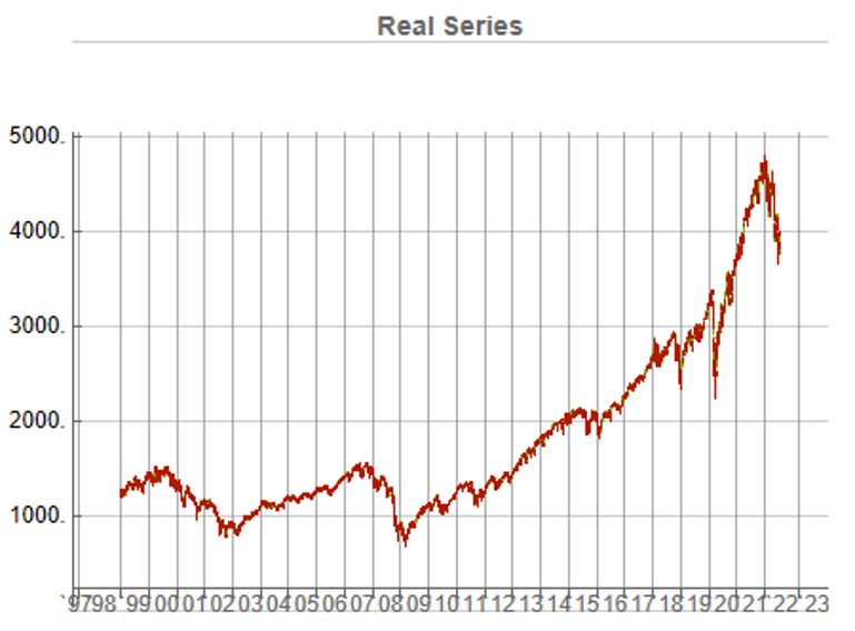
To illustrate this I will use synthetic daily data to develop a pairs trading strategy for the KO-PEP pair.
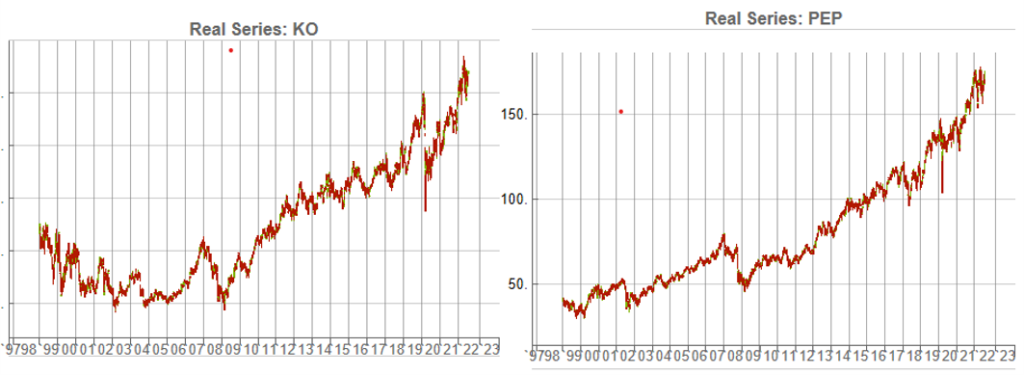
The two price series are highly correlated, which potentially makes them a suitable candidate for a pairs trading strategy.
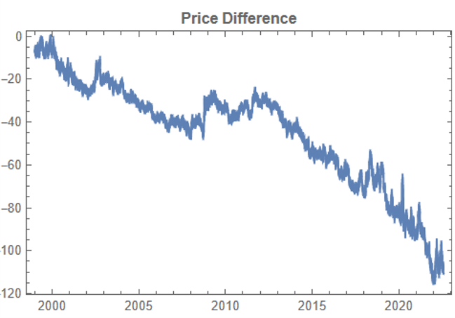
There are numerous ways to trade a pairs spread such as dollar neutral or beta neutral, but in this example I am simply going to look at trading the price difference. This is not a true market neutral approach, nor is the price difference reliably stationary. However, it will serve the purpose of illustrating the methodology.
Obviously it is crucial that the synthetic series we create behave in a way that replicates the relationship between the two stocks, so that we can use it for strategy development and testing. Ideally we would like to see high correlations between the synthetic and original price series as well as between the pairs of synthetic price data.
We begin by using the algorithm to generate 100 synthetic daily price series for KO and PEP and examine their properties.
Correlations
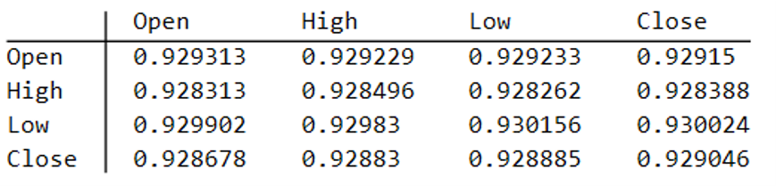
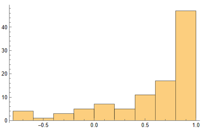
As we saw previously, the algorithm is able to generate synthetic data with correlations to the real price series ranging from below zero to close to 1.0:
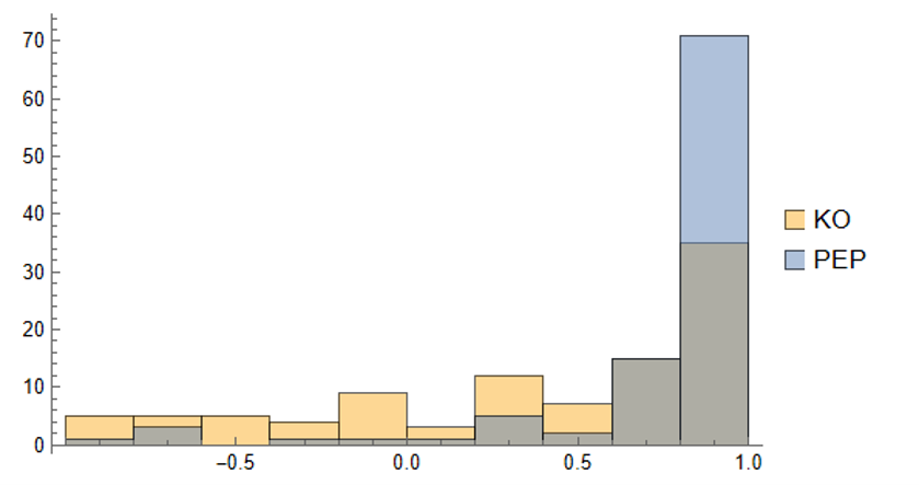
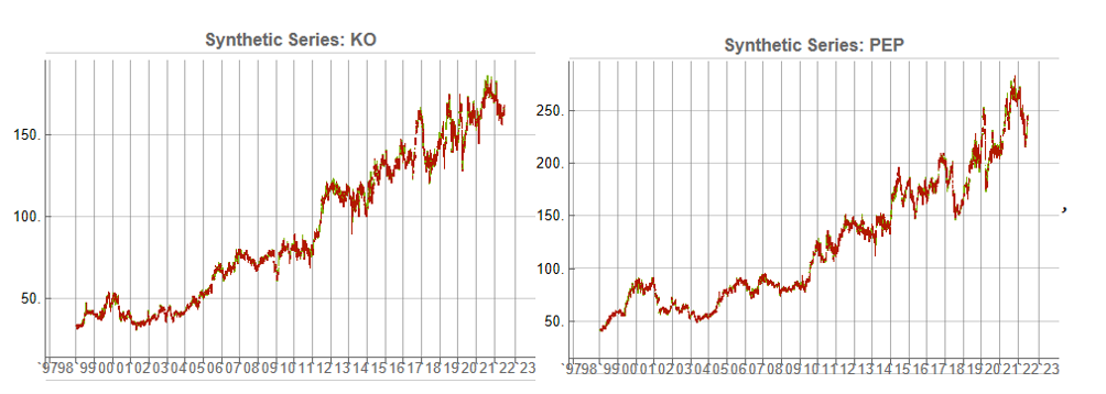
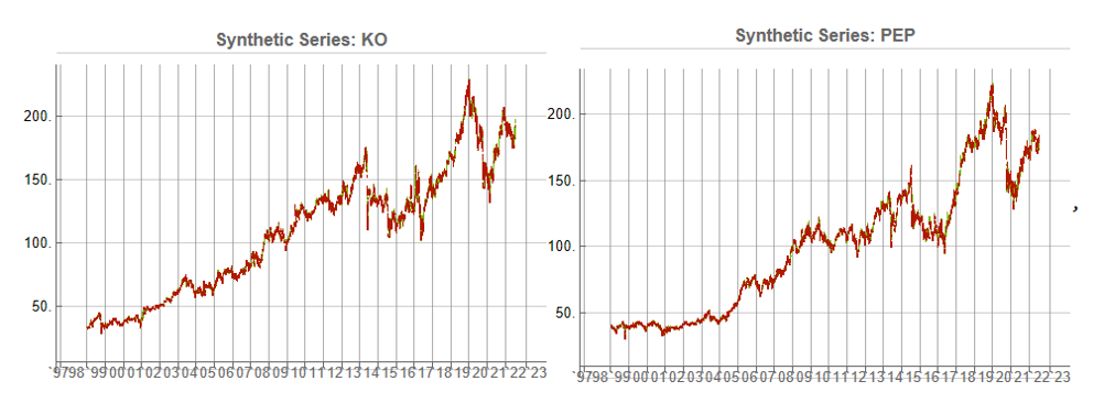
The crucial point, however, is that the algorithm has been designed to also preserve the cross-sectional correlation between the pairs of synthetic KO-PEP data, just as in the real data series:
Some examples of highly correlated pairs of synthetic data are shown in the plots below:
In addition to correlation, we might also want to consider the price differences between the pairs of synthetic series, since the strategy will be trading that price difference, in the simple approach adopted here. We could, for example, select synthetic pairs for which the divergence in the price difference does not become too large, on the assumption that the series difference is stationary. While that approach might well be reasonable in other situations, here an assumption of stationarity would be perhaps closer to wishful thinking than reality. Instead we can use of selection of synthetic pairs with high levels of cross-correlation, as we all high levels of correlation with the real price data. We can also select for high correlation between the price differences for the real and synthetic price series.
Strategy Development & WFO Testing
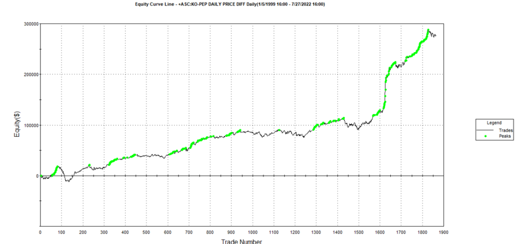
Once again we follow the procedure for strategy development outline in the previous post, except that, in addition to a selection of synthetic price difference series we also include 14-day correlations between the pairs. We use synthetic daily synthetic data from 1999 to 2012 to build the strategy and use the data from 2013 onwards for testing/validation. Eventually, after 50 generations we arrive at the result shown in the figure below:
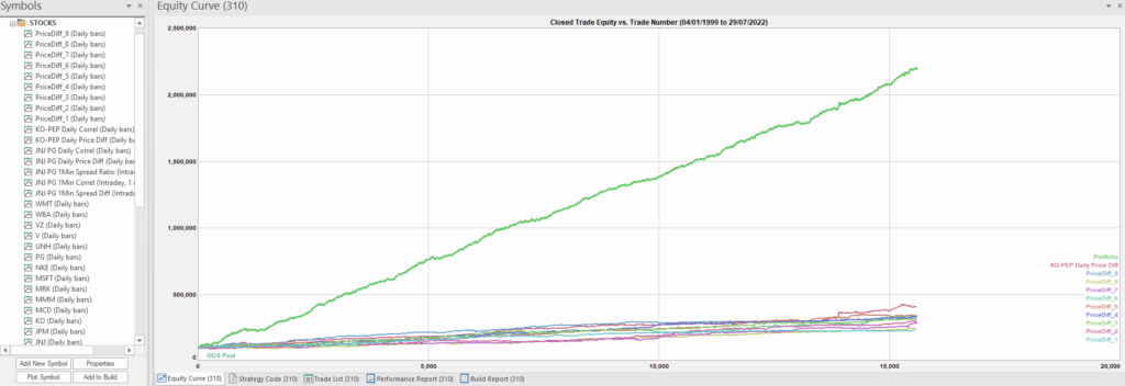
As before, the equity curve for the individual synthetic pairs are shown towards the bottom of the chart, while the aggregate equity curve, which is a composition of the results for all none synthetic pairs is shown above in green. Clearly the results appear encouraging.
As a final step we apply the WFO analysis procedure described in the previous post to test the performance of the strategy on the real data series, using a variable number in-sample and out-of-sample periods of differing size. The results of the WFO cluster test are as follows:
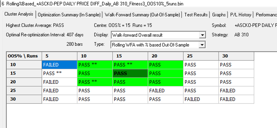
The results are no so unequivocal as for the strategy developed for the S&P 500 index, but would nonethless be regarded as acceptable, since the strategy passes the great majority of the tests (in addition to the tests on synthetic pairs data).
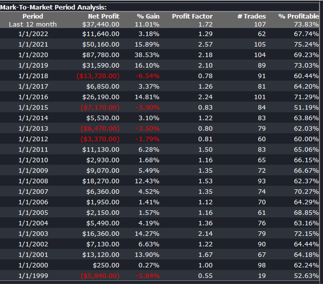
The final results appear as follows:
Conclusion
We have demonstrated how the algorithm can be used to generate synthetic price series the preserve not only the important time series properties, but also the cross-sectional properties between series for correlated securities. This important feature has applications in the development of statistical arbitrage strategies, portfolio construction methodology and in portfolio risk management.
Developing Trading Strategies With Synthetic Data

One of the main criticisms levelled at systematic trading over the last few years is that the over-use of historical market data has tended to produce curve-fitted strategies that perform poorly out of sample in a live trading environment. This is indeed a valid criticism – given enough attempts one is bound to arrive eventually at a strategy that performs well in backtest, even on a holdout data sample. But that by no means guarantees that the strategy will continue to perform well going forward.
The solution to the problem has been clear for some time: what is required is a method of producing synthetic market data that can be used to build a strategy and test it under a wide variety of simulated market conditions. A strategy built in this way is more likely to survive the challenge of live trading than one that has been developed using only a single historical data path.
The problem, however, has been in implementation. Up until now all the attempts to produce credible synthetic price data have failed, for one reason or another, as I described in an earlier post:
I have been able to devise a completely new algorithm for generating artificial price series that meet all of the key requirements, as follows:
- Computational simplicity & efficiency. Important if we are looking to mass-produce synthetic series for a large number of assets, for a variety of different applications. Some deep learning methods would struggle to meet this requirement, even supposing that transfer learning is possible.
- The ability to produce price series that are internally consistent (i.e High > Low, etc) in every case .
- Should be able to produce a range of synthetic series that vary widely in their correspondence to the original price series. In some case we want synthetic price series that are highly correlated to the original; in other cases we might want to test our investment portfolio or risk control systems under extreme conditions never before seen in the market.
- The distribution of returns in the synthetic series should closely match the historical series, being non-Gaussian and with “fat-tails”.
- The ability to incorporate long memory effects in the sequence of returns.
- The ability to model GARCH effects in the returns process.
This means that we are now in a position to develop trading strategies without any direct reference to the underlying market data. Consequently we can then use all of the real market data for out-of-sample back-testing.
Developing a Trading Strategy for the S&P 500 Index Using Synthetic Market Data
To illustrate the procedure I am going to use daily synthetic price data for the S&P 500 Index over the period from Jan 1999 to July 2022. Details of the the characteristics of the synthetic series are given in the post referred to above.
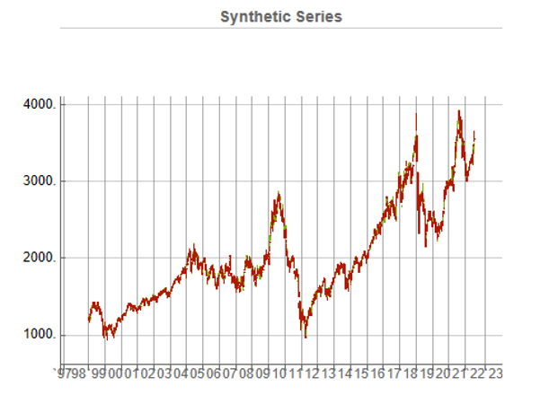
Because we want to create a trading strategy that will perform under market conditions close to those currently prevailing, I will downsample the synthetic series to include only those that correlate quite closely, i.e. with a minimum correlation of 0.75, with the real price data.
Why do this? Surely if we want to make a strategy as robust as possible we should use all of the synthetic data series for model development?
The reason is that I believe that some of the more extreme adverse scenarios generated by the algorithm may occur quite rarely, perhaps once in every few decades. However, I am principally interested in a strategy that I can apply under current market conditions and I am prepared to take my chances that the worst-case scenarios are unlikely to come about any time soon. This is a major design decision, one that you may disagree with. Of course, one could make use of every available synthetic data series in the development of the trading model and by doing so it is likely that you would produce a model that is more robust. But the training could take longer and the performance during normal market conditions may not be as good.
Having generated the price series, the process I am going to follow is to use genetic programming to develop trading strategies that will be evaluated on all of the synthetic data series simultaneously. I will then use the performance of the aggregate portfolio, i.e. the outcome of all of the trades generated by the strategy when applied to all of the synthetic series, to assess the overall performance. In order to be considered, candidate strategies have to perform well under all of the different market scenarios, or at least the great majority of them. This ensures that the strategy is likely to prove more robust across different types of market conditions, rather than on just the single type of market scenario observed in the real historical series.
As usual in these cases I will reserve a portion (10%) of each data series for testing each strategy, and a further 10% sample for out-of-sample validation. This isn’t strictly necessary: since the real data series has not be used directly in the development of the trading system, we can later test the strategy on all of the historical data and regard this as an out-of-sample backtest.
To implement the procedure I am going to use Mike Bryant’s excellent Adaptrade Builder software.
This is an exemplar of outstanding software engineering and provides a broad range of features for generating trading strategies of every kind. One feature of Builder that is particularly useful in this context is its ability to construct strategies and test them on up to 20 data series concurrently. This enables us to develop a strategy using all of the synthetic data series simultaneously, showing the performance of each individual strategy as well for as the aggregate portfolio.
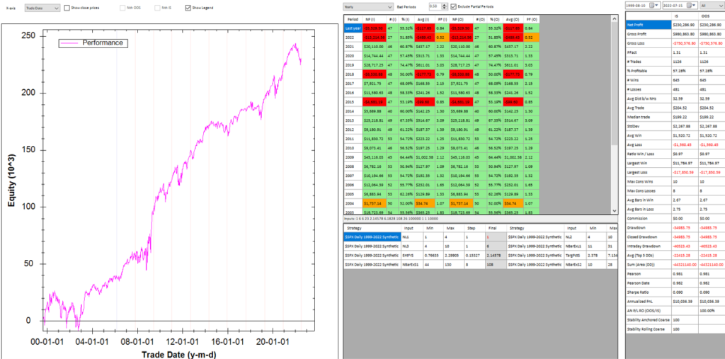
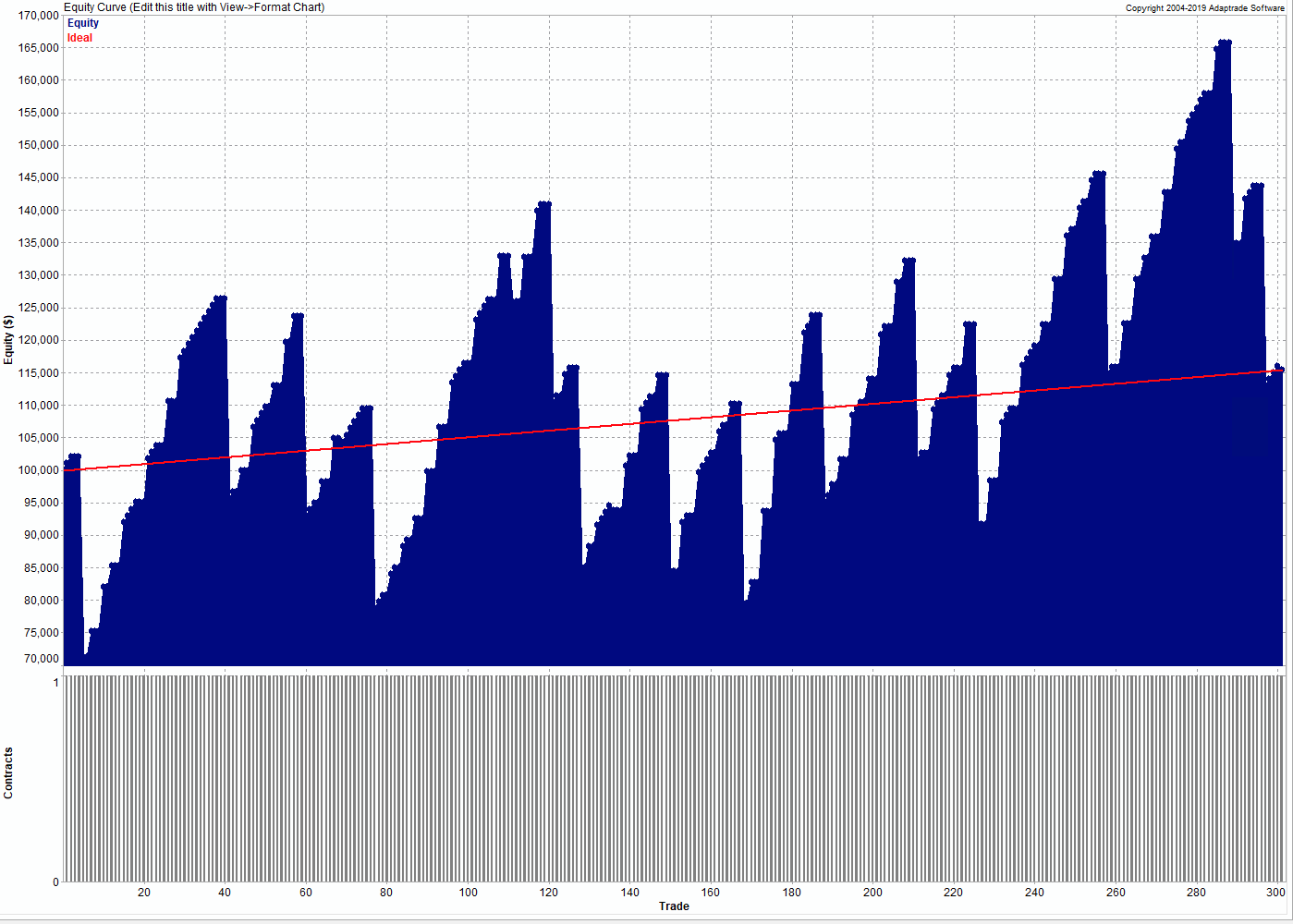
After evolving strategies for 50 generations we arrive at the following outcome:
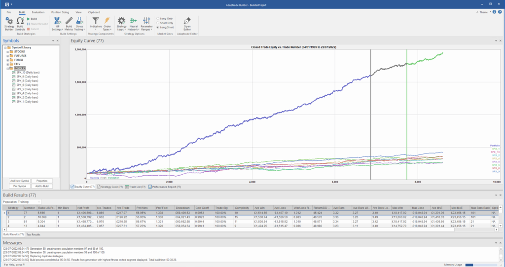
The equity curve for the aggregate portfolio is shown in blue, while the equity curves for the strategy applied to individual synthetic data series are shown towards the bottom of the chart. Of course, the performance of the aggregate portfolio appears much superior to any of the individual strategies, because it is effectively the arithmetic sum of the individual equity curves. And just because the aggregate portfolio appears to perform well both in-sample and out-of-sample, that doesn’t imply that the strategy works equally well for every individual market scenario. In some scenarios it performs better than in others, as can be observed from the individual equity curves.
But, in any case, our objective here is not to create a stock portfolio strategy, but rather to trade a single asset – the S&P 500 Index. The role of the aggregate portfolio is simply to suggest that we may have found a strategy that is sufficiently robust to work well across a variety of market conditions, as represented by the various synthetic price series.
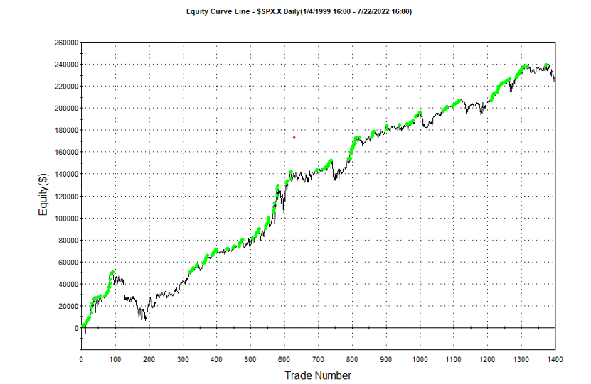
Builder generates code for the strategies it evolves in a number of different languages and in this case we take the EasyLanguage code for the fittest strategy #77 and apply it to a daily chart for the S&P 500 Index – i.e. the real data series – in Tradestation, with the following results:
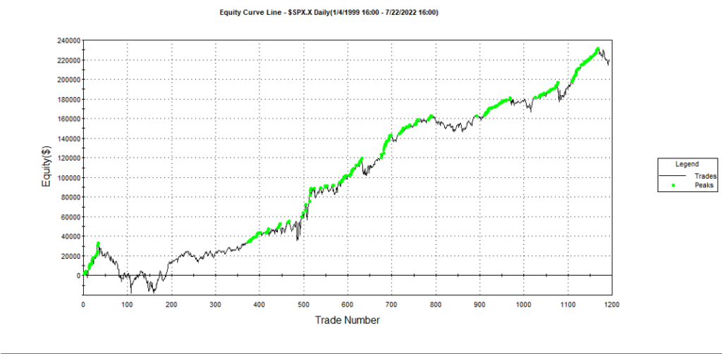
The strategy appears to work well “out-of-the-box”, i,e, without any further refinement. So our quest for a robust strategy appears to have been quite successful, given that none of the 23-year span of real market data on which the strategy was tested was used in the development process.
We can take the process a little further, however, by “optimizing” the strategy. Traditionally this would mean finding the optimal set of parameters that produces the highest net profit on the test data. But this would be curve fitting in the worst possible sense, and is not at all what I am suggesting.
Instead we use a procedure known as Walk Forward Optimization (WFO), as described in this post:
The goal of WFO is not to curve-fit the best parameters, which would entirely defeat the object of using synthetic data. Instead, its purpose is to test the robustness of the strategy. We accomplish this by using a sequence of overlapping in-sample and out-of-sample periods to evaluate how well the strategy stands up, assuming the parameters are optimized on in-sample periods of varying size and start date and tested of similarly varying out-of-sample periods. A strategy that fails a cluster of such tests is unlikely to prove robust in live trading. A strategy that passes a test cluster at least demonstrates some capability to perform well in different market regimes.
To some extent we might regard such a test as unnecessary, given that the strategy has already been observed to perform well under several different market conditions, encapsulated in the different synthetic price series, in addition to the real historical price series. Nonetheless, we conduct a WFO cluster test to further evaluate the robustness of the strategy.
As the goal of the procedure is not to maximize the theoretical profitability of the strategy, but rather to evaluate its robustness, we select a criterion other than net profit as the factor to optimize. Specifically, we select the sum of the areas of the strategy drawdowns as the quantity to minimize (by maximizing the inverse of the sum of drawdown areas, which amounts to the same thing). This requires a little explanation.
If we look at the strategy drawdown periods of the equity curve, we observe several periods (highlighted in red) in which the strategy was underwater:
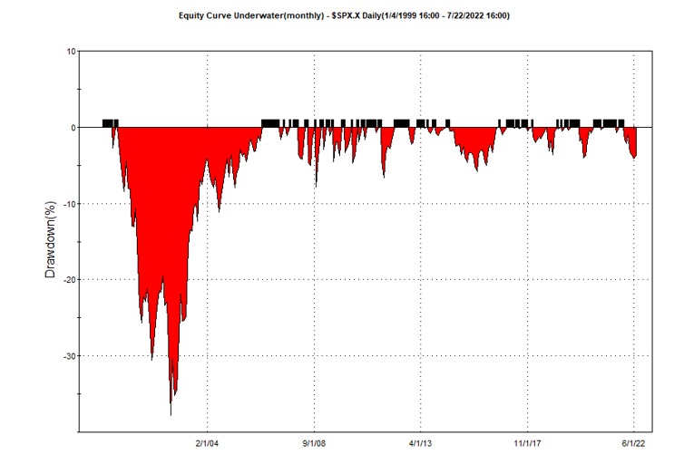
The area of each drawdown represents the length and magnitude of the drawdown and our goal here is to minimize the sum of these areas, so that we reduce both the total duration and severity of strategy drawdowns.
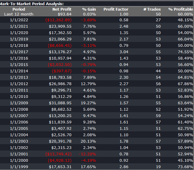
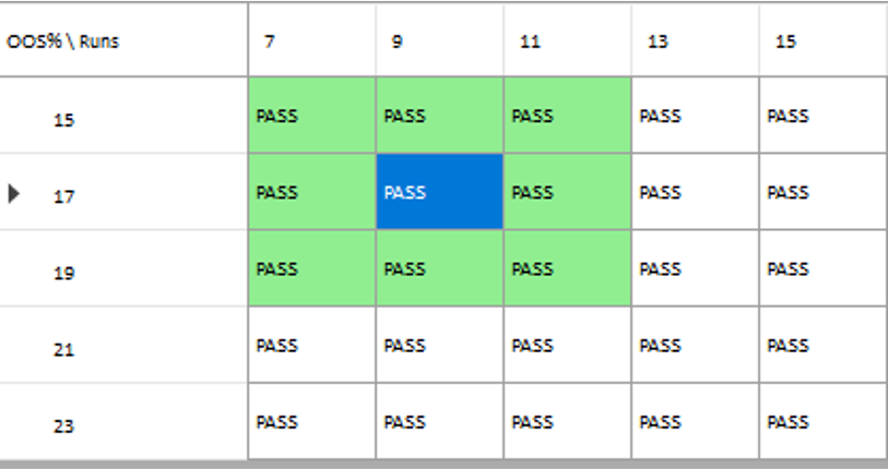
In each WFO test we use different % of OOS data and a different number of runs, assessing the performance of the strategy on a battery of different criteria:
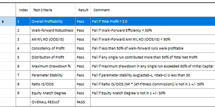
These criteria not only include overall profitability, but also factors such as parameter stability, profit consistency in each test, the ratio of in-sample to out-of-sample profits, etc. In other words, this WFO cluster analysis is not about profit maximization, but robustness evaluation, as assessed by these several different metrics. And in this case the strategy passes every test with flying colors:
Other than validating the robustness of the strategy’s performance, the overall effect of the procedure is to slightly improve the equity curve by diminishing the magnitude and duration of the drawdown periods:
Conclusion
We have shown how, by using synthetic price series, we can build a robust trading strategy that performs well under a variety of different market conditions, including on previously “unseen” historical market data. Further analysis using cluster WFO tests strengthens the assessment of the strategy’s robustness.
Backtest vs. Trading Reality

Kris Sidial, whose Twitter posts are often interesting, recently posted about the reality of trading profitability vs backtest performance, as follows:
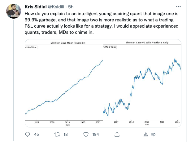
While I certainly agree that the latter example is more representative of a typical trader’s P&L, I don’t concur that the first P&L curve is necessarily “99.9% garbage”. There are many strategies that have equity curves that are smoother and more monotonic than those of Kris’s Skeleton Case V2 strategy. Admittedly, most of these lie in the area of high frequency, which is not Kris’s domain expertise. But there are also lower frequency strategies that produce results which are not dissimilar to those shown the first chart.
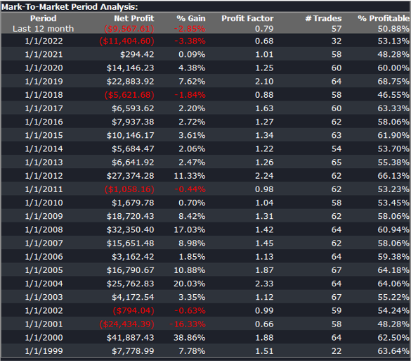
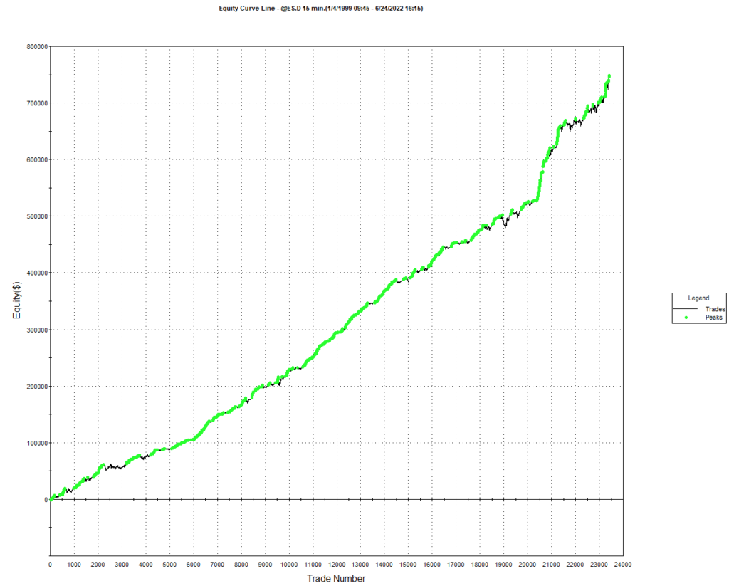
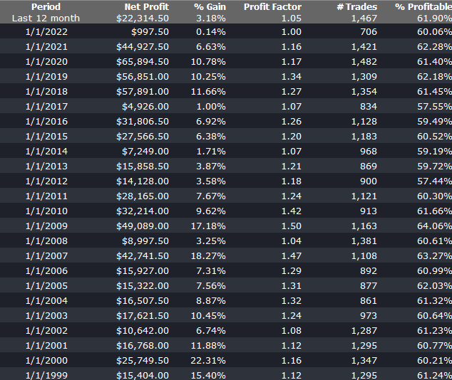
As a case in point, consider the following strategy for the S&P 500 E-Mini futures contract, described in more detail below. The strategy was developed using 15-minute bar data from 1999 to 2012, and traded live thereafter. The live and backtest performance characteristics are almost indistinguishable, not only in terms of rate of profit, but also in regard to strategy characteristics such as the no. of trades, % win rate and profit factor.
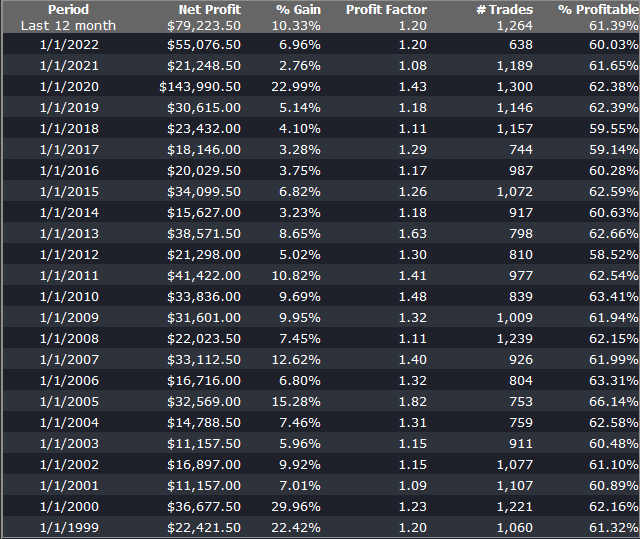
Just in case you think the picture is a little too rosy, I would point out that the average profit factor is 1.25, which means that the strategy is generating only 25% more in profits than losses. There will be big losing trades from time to time and long sequences of losses during which the strategy appears to have broken down. It takes discipline to resist the temptation to “fix” the strategy during extended drawdowns and instead rely on reversion to the mean rate of performance over the long haul. One source of comfort to the trader through such periods is that the 60% win rate means that the majority of trades are profitable.
As you read through the replies to Kris’s post, you will see that several of his readers make the point that strategies with highly attractive equity curves and performance characteristics are typically capital constrained. This is true in the case of this strategy, which I trade with a very modest amount of (my own) capital. Even trading one-lots in the E-Mini futures I occasionally experience missed trades, either on entry or exit, due to limit orders not being filled at the high or low of a bar. In scaling the strategy up to something more meaningful such as a 10-lot, there would be multiple partial fills to deal with. But I think it would be a mistake to abandon a high performing strategy such as this just because of an apparent capacity constraint. There are several approaches one can explore to address the issue, which may be enough to make the strategy scalable.
Where (as here) the issue of scalability relates to the strategy fill rate on limit orders, a good starting point is to compute the extreme hit rate, which is the proportion of trades that take place at the high or low of the bar. As a rule of thumb, for strategies running on typical low frequency infrastructure an extreme hit rate of 10% or less is manageable; anything above that level quickly becomes problematic. If the extreme hit rate is very high, e.g. 25% or more, then you are going to have to pay a great deal of attention to the issues of latency and order priority to make the strategy viable in practise. Ultimately, for a high frequency market making strategy, most orders are filled at the extreme of each “bar”, so almost all of the focus in on minimizing latency and maintaining a high queue priority, with all of the attendant concerns regarding trading hardware, software and infrastructure.
Next, you need a strategy for handling missed trades. You could, for example, decide to skip any entry trades that are missed, while manually entering unfilled exit trades at the market. Or you could post market orders for both entry and exit trades if they are not filled. An extreme solution would be to substitute market-if-touched orders for limit orders in your strategy code. But this would affect all orders generated by the system, not just the 10% at the high or low of the bar and is likely to have a very adverse affect on overall profitability, especially if the average trade is low (because you are paying an extra tick on entry and exit of every trade).
The above suggests that you are monitoring the strategy manually, running simulation and live versions side by side, so that you can pick up any trades that the strategy should have taken, but which have been missed. This may be practical for a strategy that trades during regular market hours, but not for one that also trades the overnight session.
An alternative approach, one that is commonly applied by systematic traders, is to automate the handling of missed trades. Typically the trader will set a parameter that converts a limit order to a market order X seconds after a limit price has been traded but not filled. Of course, this will result in paying up an extra tick (or more) to enter trades that perhaps would have been filled if one had waited longer than X seconds. It will have some negative impact on strategy profitability, but not too much if the extreme hit rate is low. I tend to use this method for exit trades, preferring to skip any entry trades that don’t get filled at the limit price.
Beyond these simple measures, there are several other ways to extend the capacity of the strategy. An obvious place to start is by evaluating strategy performance on different session times and bar lengths. So, in this case, we might look at deploying the strategy on both the day and night sessions. We can also evaluate performance on bars of different length. This will give different entry and exit points for individual trades and trades that are at the extreme of a bar on one timeframe may not be at the high or low of a bar on the other timescale. For example, here is the (simulated) performance of the strategy on 13 minute bars:
There is a reason for choosing a bar interval such as 13 minutes, rather than the more commonplace 5- or 10 minutes, as explained in this post:
Finally, it is worth exploring whether the strategy can be applied to other related markets such as NQ futures, for example. Typically this will entail some change to the strategy code to reflect the difference in price levels, but the thrust of the strategy logic will be similar. Another approach is to use the signals from the current strategy as inputs – i.e. alpha generators – for a derivative strategy, such as trading the SPY ETF based on signals from the ES strategy. The performance of the derived strategy may not be as good, but in a product like SPY the capacity might be larger.
Master’s in High Frequency Finance

I have been discussing with some potential academic partners the concept for a new graduate program in High Frequency Finance. The idea is to take the concept of the Computational Finance program developed in the 1990s and update it to meet the needs of students in the 2010s.
The program will offer a thorough grounding in the modeling concepts, trading strategies and risk management procedures currently in use by leading investment banks, proprietary trading firms and hedge funds in US and international financial markets. Students will also learn the necessary programming and systems design skills to enable them to make an effective contribution as quantitative analysts, traders, risk managers and developers.
I would be interested in feedback and suggestions as to the proposed content of the program.
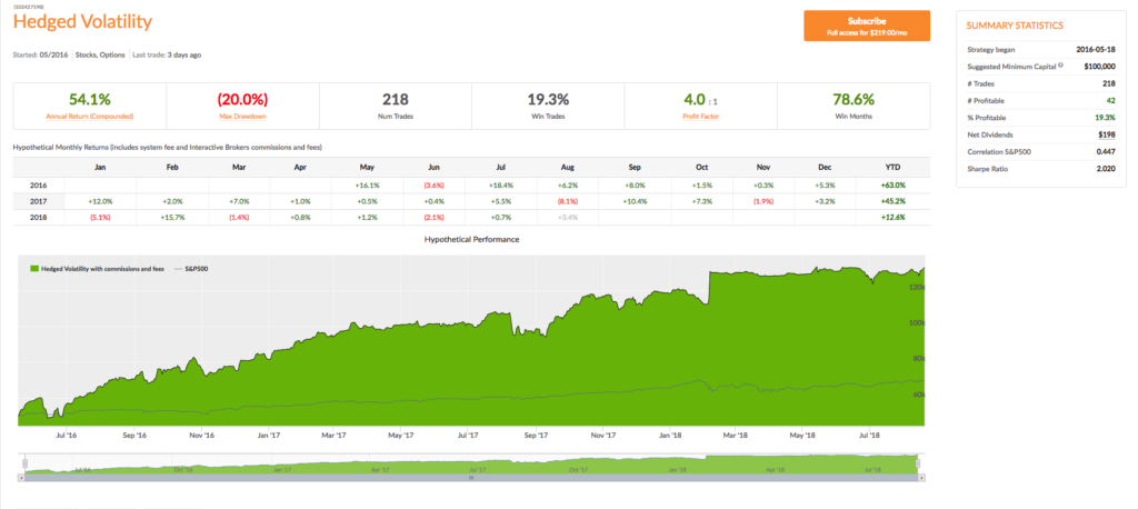
The Hedged Volatility Strategy

Being short regular Volatility ETFs or long Inverse Volatility ETFs are winning strategies…most of the time. The challenge is that when the VIX spikes or when the VIX futures curve is downward sloping instead of upward sloping, very significant losses can occur. Many people have built and back-tested models that attempt to move from long to short to neutral positions in the various Volatility ETFs, but almost all of them have one or both of these very significant flaws: 1) Failure to use “out of sample” back-testing and 2) Failure to protect against “black swan” events.
In this strategy a position and weighting in the appropriate Volatility ETFs are established based on a multi-factor model which always uses out of sample back-testing to determine effectiveness. Volatility Options are always used to protect against significant short-term moves which left unchecked could result in the total loss of one’s portfolio value; these options will usually lose money, but that is a small price to pay for the protection they provide. (Strategies should be scaled at a minimum of 20% to ensure options protection.)
This is a good strategy for IRA accounts in which short selling is not allowed. Long positions in Inverse Volatility ETFs are typically held. Suggested minimum capital: $26,000 (using 20% scaling).
A Meta-Strategy in S&P 500 E-Mini Futures

In earlier posts I have described the idea of a meta-strategy as a strategies that trades strategies. It is an algorithm, or set of rules, that is used to decide when to trade an underlying strategy. In some cases a meta-strategy may influence the size in which the underlying strategy is traded, or may even amend the base code. In other word, a meta-strategy actively “trades” an underlying strategy, or group of strategies, much as in the same way a regular strategy may actively trade stocks, going long or short from time to time. One distinction is that a meta-strategy will rarely, if ever, actually “short” an underlying strategy – at most it will simply turn the strategy off (reduce the position size to zero) for a period.
For a more detailed description, see this post:
In this post I look at a meta-strategy that developed for a client’s strategy in S&P E-Mini futures. What is extraordinary is that the underlying strategy was so badly designed (not by me!) and performs so poorly that no rational systematic trader would likely give it a second look – instead he would toss it into the large heap of failed ideas that all quantitative researchers accumulate over the course of their careers. So this is a textbook example that illustrates the power of meta-strategies to improve, or in this case transform, the performance of an underlying strategy.
1. The Strategy
The Target Trader Strategy (“TTS”) is a futures strategy applied to S&P 500 E-Mini futures that produces a very high win rate, but which occasionally experiences very large losses. The purpose of the analysis if to find methods that will:
1) Decrease the max loss / drawdown
2) Increase the win rate / profitability
For longs the standard setting is entry 40 ticks below the target, stop loss 1000 ticks below the target, and then 2 re-entries 100 ticks below entry 1 and 100 ticks below entry 2
For shorts the standard is entry 80 ticks above the target. stop loss 1000 ticks above the target, and then 2 re-entries 100 ticks above entry 1 and 100 ticks above entry 2
For both directions its 80 ticks above/below for entry 1, 1000 tick stop, and then 1 re entry 100 ticks above/below, and then re-entry 2 100 ticks above/below entry 2
2. Strategy Performance
2.1 Overall Performance
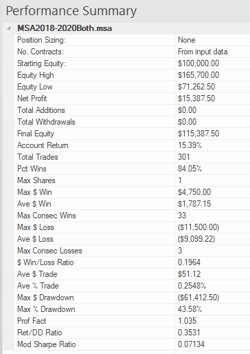
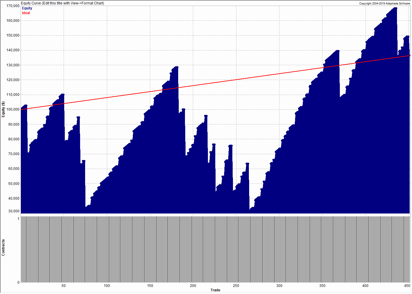
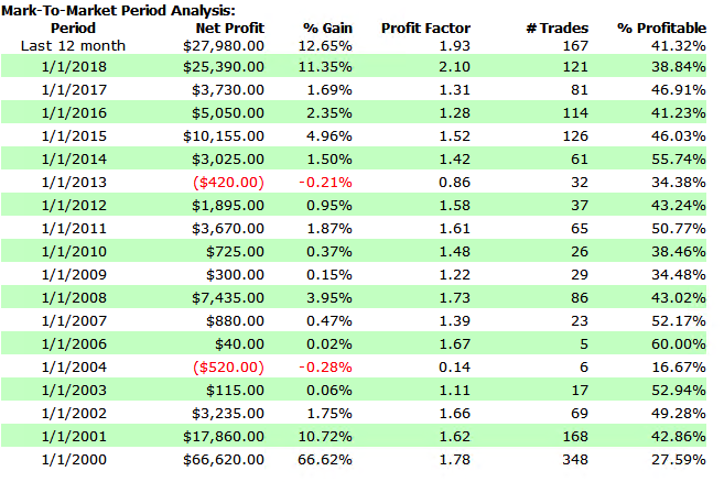
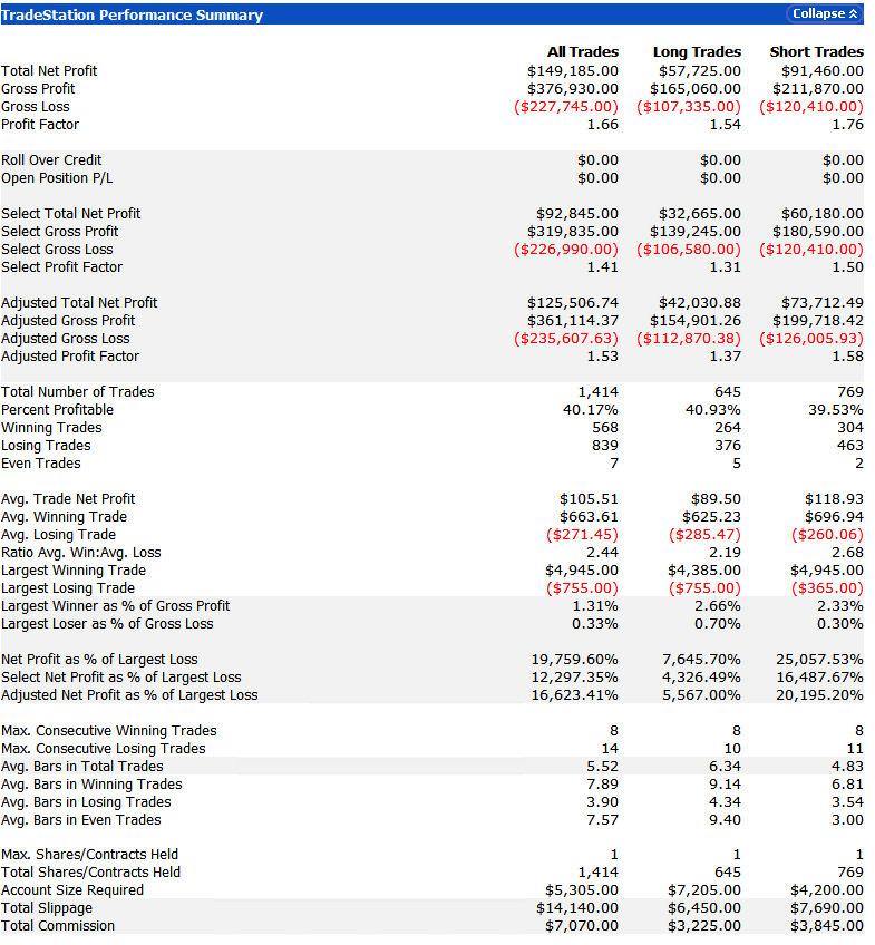
The overall performance of the strategy over the period from 2018 to 2020 is summarized in the chart of the strategy equity curve and table of performance statistics below.
These confirm that, while the win rate if very high (over 84%) there strategy experiences many significant drawdowns, including a drawdown of -$61,412.50 (-43.58%). The total return is of the order of 5% per year, the strategy profit factor is fractionally above 1 and the Sharpe Ratio is negligibly small. Many traders would consider the performance to be highly unattractive.
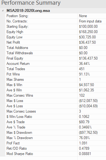
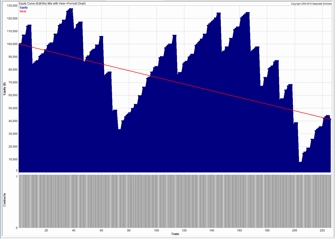
2.2 Long Trades
We break the strategy performance down into long and short trades, and consider them separately. On the long side, the strategy has been profitable, producing a gain of over 36% during the period 2018-2020. It also suffered catastrophic drawdown of over -$97,000 during that period:
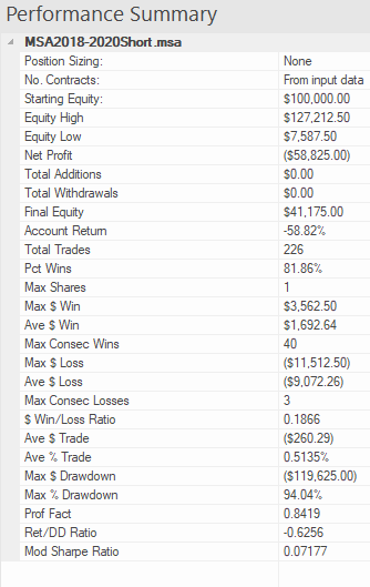
2.3 Short Trades
On the short side, the story is even worse, producing an overall loss of nearly -$59,000:
3. Improving Strategy Performance with a Meta-Strategy
We considered two possible methods to improve strategy performance. The first method attempts to apply technical indicators and other data series to improve trading performance. Here we evaluated price series such as the VIX index and a wide selection of technical indicators, including RSI, ADX, Moving Averages, MACD, ATR and others. However, any improvement in strategy performance proved to be temporary in nature and highly variable, in many cases amplifying the problems with the strategy performance rather than improving them.
The second approach proved much more effective, however. In this method we create a meta-strategy which effectively “trades the strategy”, turning it on and off depending on its recent performance. The meta-strategy consists of a set of rules that determines whether or not to continue trading the strategy after a series of wins or losses. In some cases the meta-strategy may increase the trade size for a sequence of trades, at times when it considers the conditions for the underlying strategy to be favorable.
The result of applying the meta-strategy are described in the following sections.
3.1 Long & Short Strategies with Meta-Strategy Overlay
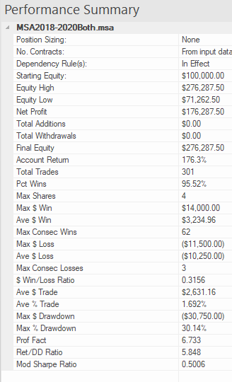
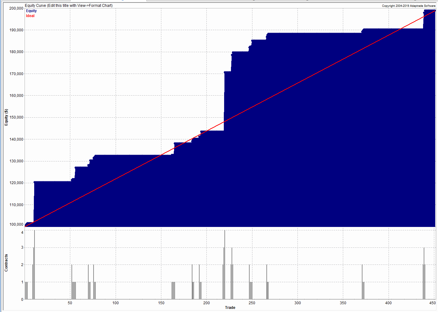
The performance of the long/short strategies combined with the meta-strategy overlay are set out in the chart and table below.
The overall improvements can be summarized as follows:
- Net profit increases from $15,387 to $176,287
- Account return rises from 15% to 176%
- Percentage win rate rises from 84% to 95%
- Profit factor increases from 1.0 to 6.7
- Average trade rises from $51 to $2,631
- Max $ Drawdown falls from -$61,412 to -$30,750
- Return/Max Drawdown ratio rises from 0.35 to 5.85
- The modified Sharpe ratio increases from 0.07 to 0.5
Taken together, these are dramatic improvements to every important aspect of strategy performance.
There are two key rules in the meta-strategy, applicable to winning and losing trades:
Rule for winning trades:
After 3 wins in a row, skip the next trade.
Rule for losing trades:
After 3 losses in a row, add 1 contract until the first win. Subtract 1 contract after each win until the next loss, or back to 1 contract.
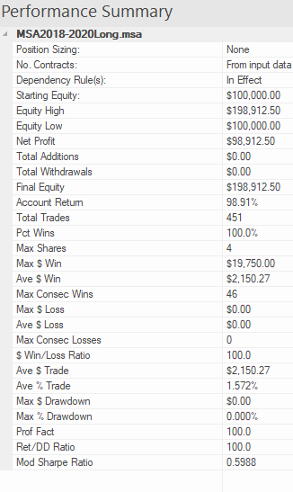
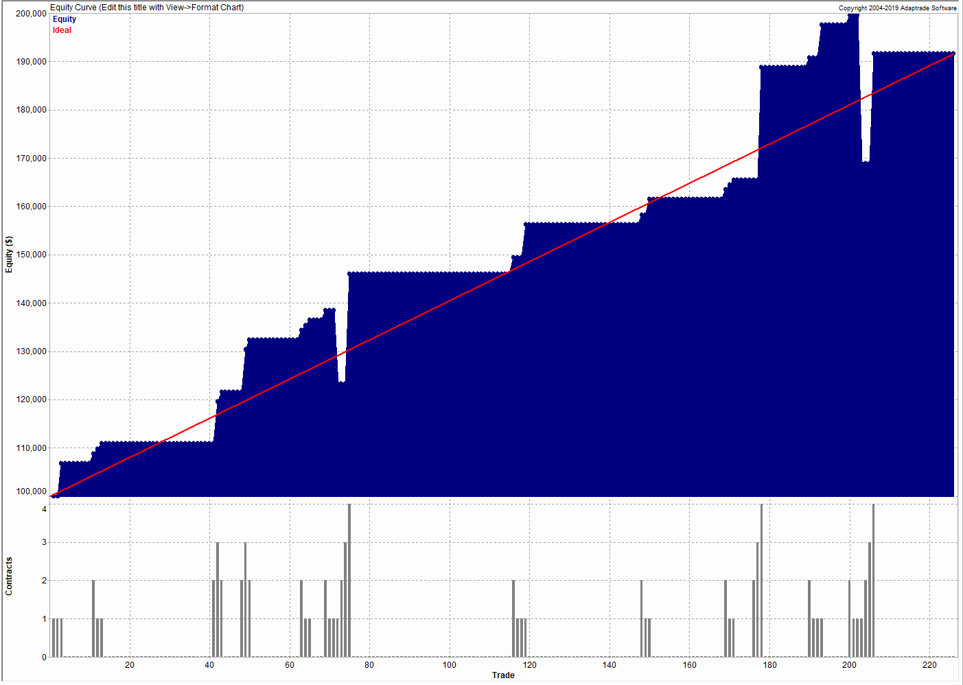
3.2 Long Trades with Meta-Strategy
The meta-strategy rules produce significant improvements in the performance of both the long and short components of the strategy. On the long side the percentage win rate is increased to 100% and the max % drawdown is reduced to 0%:
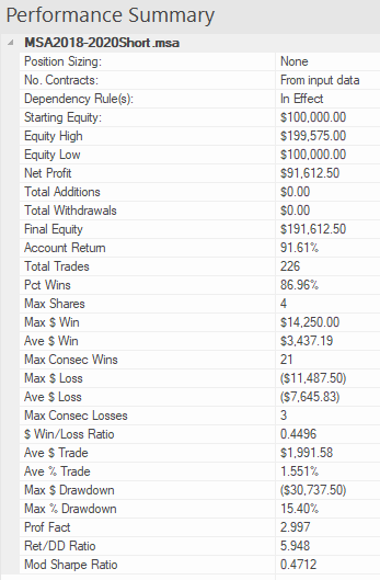
3.3 Short Trades with Meta-Strategy
Improvements to the strategy on the short side are even more significant, transforming a loss of -$59,000 into a profit of $91,600:
4. Conclusion
A meta-strategy is a simple, yet powerful technique that can transform the performance of an underlying strategy. The rules are often simple, although they can be challenging to implement. Meta strategies can be applied to almost any underlying strategy, whether in futures, equities, or forex. Worthwhile improvements in strategy performance are often achievable, although not often as spectacular as in this case.
If any reader is interested in designing a meta-strategy for their own use, please get in contact.
Career Opportunity for Quant Traders

Career Opportunity for Quant Traders as Strategy Managers
We are looking for 3-4 traders (or trading teams) to showcase as Strategy Managers on our Algorithmic Trading Platform. Ideally these would be systematic quant traders, since that is the focus of our fund (although they don’t have to be). So far the platform offers a total of 10 strategies in equities, options, futures and f/x. Five of these are run by external Strategy Managers and five are run internally.
The goal is to help Strategy Managers build a track record and gain traction with a potential audience of over 100,000 members. After a period of 6-12 months we will offer successful managers a position as a PM at Systematic Strategies and offer their strategies in our quantitative hedge fund. Alternatively, we will assist the manager is raising external capital in order to establish their own fund.
If you are interested in the possibility (or know a talented rising star who might be), details are given below.

Daytrading Index Futures Arbitrage

Trading with Indices
I have always been an advocate of incorporating index data into one’s trading strategies. Since they are not tradable, the “market” in index products if often highly inefficient and displays easily identifiable patterns that can be exploited by a trader, or a trading system. In fact, it is almost trivially easy to design “profitable” index trading systems and I gave a couple of examples in the post below, including a system producing stellar results in the S&P 500 Index.
http://jonathankinlay.com/2016/05/trading-with-indices/
Of course such systems are not directly useful. But traders often use signals from such a system as a filter for an actual trading system. So, for example, one might look for a correlated signal in the S&P 500 index as a means of filtering trades in the E-Mini futures market or theSPDR S&P 500 ETF (SPY).
Multi-Strategy Trading Systems
This is often as far as traders will take the idea, since it quickly gets a lot more complicated and challenging to build signals generated from an index series into the logic of a strategy designed for related, tradable market. And for that reason, there is a great deal of unexplored potential in using index data in this way. So, for instance, in the post below I discuss a swing trading system in the S&P500 E-mini futures (ticker: ES) that comprises several sub-systems build on prime-valued time intervals. This has the benefit of minimizing the overlap between signals from multiple sub-systems, thereby increasing temporal diversification.
http://jonathankinlay.com/2018/07/trading-prime-market-cycles/
A critical point about this system is that each of sub-systems trades the futures market based on data from both the E-mini contract and the S&P 500 cash index. A signal is generated when the system finds particular types of discrepancy between the cash index and corresponding futures, in a quasi risk-arbitrage.

Arbing the NASDAQ 100 Index Futures
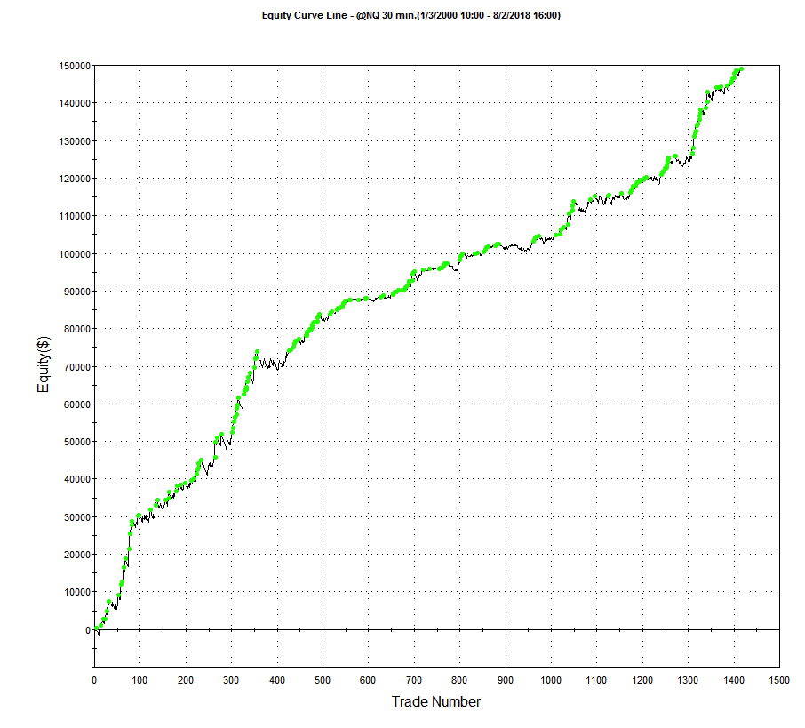
Developing trading systems for the S&P500 E-mini futures market is not that hard. A much tougher challenge, at least in my experience, is presented by the E-mini NASDAQ-100 futures (ticker: NQ). This is partly to do with the much smaller tick size and different market microstructure of the NASDAQ futures market. Additionally, the upward drift in equity related products typically favors strategies that are long-only. Where a system trades both long and short sides of the market, the performance on the latter is usually much inferior. This can mean that the strategy performs poorly in bear markets such as 2008/09 and, for the tech sector especially, the crash of 2000/2001. Our goal was to develop a daytrading system that might trade 1-2 times a week, and which would perform as well or better on short trades as on the long side. This is where NASDAQ 100 index data proved to be especially helpful. We found that discrepancies between the cash index and futures market gave particularly powerful signals when markets seemed likely to decline. Using this we were able to create a system that performed exceptionally well during the most challenging market conditions. It is notable that, in the performance results below (for a single futures contract, net of commissions and slippage), short trades contributed the greater proportion of total profits, with a higher overall profit factor and average trade size.
Conclusion: Using Index Data, Or Other Correlated Signals, Often Improves Performance
It is well worthwhile investigating how non-tradable index data can be used in a trading strategy, either as a qualifying signal or, more directly, within the logic of the algorithm itself. The greater challenge of building such systems means that there are opportunities to be found, even in well-mined areas like index futures markets. A parallel idea that likewise offers plentiful opportunity is in designing systems that make use of data on multiple time frames, and in correlated markets, for instance in the energy sector.Here one can identify situations in which, under certain conditions, one market has a tendency to lead another, a phenomenon referred to as Granger Causality.