Using Volatility to Predict Market Direction

Decomposing Asset Returns


We can decompose the returns process Rt as follows:

While the left hand side of the equation is essentially unforecastable, both of the right-hand-side components of returns display persistent dynamics and hence are forecastable. Both the signs of returns and magnitude of returns are conditional mean dependent and hence forecastable, but their product is conditional mean independent and hence unforecastable. This is an example of a nonlinear “common feature” in the sense of Engle and Kozicki (1993).

Although asset returns are essentially unforecastable, the same is not true for asset return signs (i.e. the direction-of-change). As long as expected returns are nonzero, one should expect sign dependence, given the overwhelming evidence of volatility dependence. Even in assets where expected returns are zero, sign dependence may be induced by skewness in the asset returns process.  Hence market timing ability is a very real possibility, depending on the relationship between the mean of the asset returns process and its higher moments. The highly nonlinear nature of the relationship means that conditional sign dependence is not likely to be found by traditional measures such as signs autocorrelations, runs tests or traditional market timing tests. Sign dependence is likely to be strongest at intermediate horizons of 1-3 months, and unlikely to be important at very low or high frequencies. Empirical tests demonstrate that sign dependence is very much present in actual US equity returns, with probabilities of positive returns rising to 65% or higher at various points over the last 20 years. A simple logit regression model captures the essentials of the relationship very successfully.

Now consider the implications of dependence and hence forecastability in the sign of asset returns, or, equivalently, the direction-of-change. It may be possible to develop profitable trading strategies if one can successfully time the market, regardless of whether or not one is able to forecast the returns themselves.  

There is substantial evidence that sign forecasting can often be done successfully. Relevant research on this topic includes Breen, Glosten and Jaganathan (1989), Leitch and Tanner (1991), Wagner, Shellans and Paul (1992), Pesaran and Timmerman (1995), Kuan and Liu (1995), Larsen and Wozniak (10050, Womack (1996), Gencay (1998), Leung Daouk and Chen (1999), Elliott and Ito (1999) White (2000), Pesaran and Timmerman (2000), and Cheung, Chinn and Pascual (2003).

There is also a huge body of empirical research pointing to the conditional dependence and forecastability of asset volatility. Bollerslev, Chou and Kramer (1992) review evidence in the GARCH framework, Ghysels, Harvey and Renault (1996) survey results from stochastic volatility modeling, while Andersen, Bollerslev and Diebold (2003) survey results from realized volatility modeling.

Sign Dynamics Driven By Volatility Dynamics

Let the returns process Rt be Normally distributed with mean m and conditional volatility st.

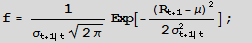
The probability of a positive return Pr[Rt+1 >0] is given by the Normal CDF F=1-Prob[0,f]


For a given mean return, m, the probability of a positive return is a function of conditional volatility st. As the conditional volatility increases, the probability of a positive return falls, as illustrated in Figure 1 below with m = 10% and st = 5% and 15%.

In the former case, the probability of a positive return is greater because more of the probability mass lies to the right of the origin. Despite having the same, constant expected return of 10%, the process has a greater chance of generating a positive return in the first case than in the second. Thus volatility dynamics drive sign dynamics.  
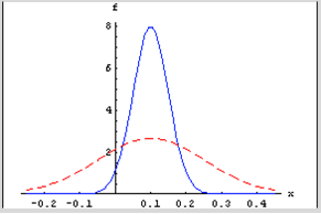
 Figure 1

Email me at jkinlay@investment-analytics.com.com for a copy of the complete article.


Volatility Metrics

Volatility Estimation

For a very long time analysts were content to accept the standard deviation of returns as the norm for estimating volatility, even though theoretical research and empirical evidence dating from as long ago as 1980 suggested that superior estimators existed.
Part of the reason was that the claimed efficiency improvements of the Parkinson, GarmanKlass and other estimators failed to translate into practice when applied to real data. Or, at least, no one could quite be sure whether such estimators really were superior when applied to empirical data since volatility, the second moment of the returns distribution, is inherently unknowable. You can say for sure what the return on a particular stock in a particular month was simply by taking the log of the ratio of the stock price at the month end and beginning. But the same cannot be said of volatility: the standard deviation of daily returns during the month, often naively assumed to represent the asset volatility, is in fact only an estimate of it.

Realized Volatility

All that began to change around 2000 with the advent of high frequency data and the concept of Realized Volatility developed by Andersen and others (see Andersen, T.G., T. Bollerslev, F.X. Diebold and P. Labys (2000), “The Distribution of Exchange Rate Volatility,” Revised version of NBER Working Paper No. 6961). The researchers showed that, in principle, one could arrive at an estimate of volatility arbitrarily close to its true value by summing the squares of asset returns at sufficiently high frequency. From this point onwards, Realized Volatility became the “gold standard” of volatility estimation, leaving other estimators in the dust.

Except that, in practice, there are often reasons why Realized Volatility may not be the way to go: for example, high frequency data may not be available for the series, or only for a portion of it; and bid-ask bounce can have a substantial impact on the robustness of Realized Volatility estimates. So even where high frequency data is available, it may still make sense to compute alternative volatility estimators. Indeed, now that a “gold standard” estimator of true volatility exists, it is possible to get one’s arms around the question of the relative performance of other estimators. That was my intent in my research paper on Estimating Historical Volatility, in which I compare the performance characteristics of the Parkinson, GarmanKlass and other estimators relative to the realized volatility estimator. The comparison was made on a number of synthetic GBM processes in which the simulated series incorporated non-zero drift, jumps, and stochastic volatility. A further evaluation was made using an actual data series, comprising 5 minute returns on the S&P 500 in the period from Jan 1988 to Dec 2003.

The findings were generally supportive of the claimed efficiency improvements for all of the estimators, which were superior to the classical standard deviation of returns on every criterion in almost every case. However, the evident superiority of all of the estimators, including the Realized Volatility estimator, began to decline for processes with non-zero drift, jumps and stochastic volatility. There was even evidence of significant bias in some of the estimates produced for some of the series, notably by the standard deviation of returns estimator.

The Log Volatility Estimator

Finally, analysis of the results from the study of the empirical data series suggested that there were additional effects in the empirical data, not seen in the simulated processes, that caused estimator efficiency to fall well below theoretical levels. One conjecture is that long memory effects, a hallmark of most empirical volatility processes, played a significant role in that finding.
The bottom line is that, overall, the log-range volatility estimator performs robustly and with superior efficiency to the standard deviation of returns estimator, regardless of the precise characteristics of the underlying process.

Estimating Historical Volatility

Career Opportunity for Quant Traders

Career Opportunity for Quant Traders as Strategy Managers

We are looking for 3-4 traders (or trading teams) to showcase as Strategy Managers on our Algorithmic Trading Platform.  Ideally these would be systematic quant traders, since that is the focus of our fund (although they don’t have to be).  So far the platform offers a total of 10 strategies in equities, options, futures and f/x.  Five of these are run by external Strategy Managers and five are run internally.

The goal is to help Strategy Managers build a track record and gain traction with a potential audience of over 100,000 members.  After a period of 6-12 months we will offer successful managers a position as a PM at Systematic Strategies and offer their strategies in our quantitative hedge fund.  Alternatively, we will assist the manager is raising external capital in order to establish their own fund.

If you are interested in the possibility (or know a talented rising star who might be), details are given below.

Manager Platform

Daytrading Index Futures Arbitrage

Trading with Indices

I have always been an advocate of incorporating index data into one’s trading strategies.  Since they are not tradable, the “market” in index products if often highly inefficient and displays easily identifiable patterns that can be exploited by a trader, or a trading system.  In fact, it is almost trivially easy to design “profitable” index trading systems and I gave a couple of examples in the post below, including a system producing stellar results in the S&P 500 Index.


http://jonathankinlay.com/2016/05/trading-with-indices/

Of course such systems are not directly useful.  But traders often use signals from such a system as a filter for an actual trading system.  So, for example, one might look for a correlated signal in the S&P 500 index as a means of filtering trades in the E-Mini futures market or theSPDR S&P 500 ETF (SPY).

Multi-Strategy Trading Systems

This is often as far as traders will take the idea, since it quickly gets a lot more complicated and challenging to build signals generated from an index series into the logic of a strategy designed for related, tradable market. And for that reason, there is a great deal of unexplored potential in using index data in this way.  So, for instance, in the post below I discuss a swing trading system in the S&P500 E-mini futures (ticker: ES) that comprises several sub-systems build on prime-valued time intervals.  This has the benefit of minimizing the overlap between signals from multiple sub-systems, thereby increasing temporal diversification.

http://jonathankinlay.com/2018/07/trading-prime-market-cycles/

A critical point about this system is that each of sub-systems trades the futures market based on data from both the E-mini contract and the S&P 500 cash index.  A signal is generated when the system finds particular types of discrepancy between the cash index and corresponding futures, in a quasi risk-arbitrage.

SSALGOTRADING AD

Arbing the NASDAQ 100 Index Futures

Developing trading systems for the S&P500 E-mini futures market is not that hard.  A much tougher challenge, at least in my experience, is presented by the E-mini NASDAQ-100 futures (ticker: NQ).  This is partly to do with the much smaller tick size and different market microstructure of the NASDAQ futures market. Additionally, the upward drift in equity related products typically favors strategies that are long-only.  Where a system trades both long and short sides of the market, the performance on the latter is usually much inferior.  This can mean that the strategy performs poorly in bear markets such as 2008/09 and, for the tech sector especially, the crash of 2000/2001.  Our goal was to develop a daytrading system that might trade 1-2 times a week, and which would perform as well or better on short trades as on the long side.  This is where NASDAQ 100 index data proved to be especially helpful.  We found that discrepancies between the cash index and futures market gave particularly powerful signals when markets seemed likely to decline.  Using this we were able to create a system that performed exceptionally well during the most challenging market conditions. It is notable that, in the performance results below (for a single futures contract, net of commissions and slippage), short trades contributed the greater proportion of total profits, with a higher overall profit factor and average trade size.

EC

Annual PL

PL

Conclusion: Using Index Data, Or Other Correlated Signals, Often Improves Performance

It is well worthwhile investigating how non-tradable index data can be used in a trading strategy, either as a qualifying signal or, more directly, within the logic of the algorithm itself.  The greater challenge of building such systems means that there are opportunities to be found, even in well-mined areas like index futures markets.  A parallel idea that likewise offers plentiful opportunity is in designing systems that make use of data on multiple time frames, and in correlated markets, for instance in the energy sector.Here one can identify situations in which, under certain conditions, one market has a tendency to lead another, a phenomenon referred to as Granger Causality.