
Why Synthetic Data?
Synthetic market data has great potential for applications in financial research. Examples include testing the risk characteristics of a trading book or investment portfolio, developing trading strategies using previously unseen data, or simulating high frequency trading activity in a limit order book. It provides an answer to the criticism of curve fitting that is routinely levelled at existing approaches that use the single, observed historical path followed by an asset to construct investment and risk models. Such models, critics argue, are usually over-fitted to the historical data and are consequently unlikely to prove robust, going forward.
What is required is a model of the underlying asset processes that can then be used to generate a large number of price paths for all of the constituents of an investment portfolio. This should provide a more realistic assessment of the range of possible behaviours of the portfolio under a wide variety of market conditions, including during tail events.
Existing Methodology
Current approaches to modelling asset processes are often rudimentary and fail to capture the interplay of market dynamics that impact the evolution of the process. So, for example, we might begin by modelling the process of asset returns using a Gaussian or Student-T distribution. This immediately runs into the issue of under-representing the “fat tails” of empirical asset distributions, where tail events occur much more frequently than standard distributions would suggest. We might move on consider using the empirical distribution itself, and this might be sufficient for some applications.
But in many cases we want to generate a sequence of returns, or perhaps a time series of Open/High/Low/Close prices for modelling purposes. This is a challenge that is at least an order of magnitude more difficult. We not only have to ensure that the returns and/or prices at each individual time step are consistent (e.g. that the High > Low, in the case of prices, for example), but also that the sequence of returns is representative of known characteristics of financial assets such as serial autocorrelation, cross correlation and volatility clustering. GARCH models serve reasonably well in this context, but, for example, fail to capture long memory effects, amongst other deficiencies.
Deep Learning Models
Generative Adversarial Networks have become ubiquitous in the generation of “deep fakes” – .synthesised images generated by deep learning models that are close to indistinguishable from the real thing, whether it be the image of a human face, or medical images such X-ray scans. In 2019 Jinsung Yoon, Daniel Jarrett, and Mihaela van der Schaar published a paper on Time-series Generative Adversarial Networks (“TimeGAN”) in Neural Information Processing Systems (link to paper here) , a deep learning model that can be used to generate synthetic time series data.
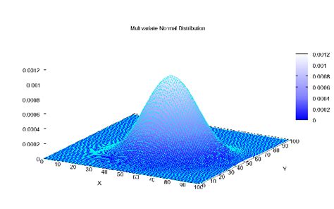
An important characteristic of time series data is that it extends regular tabular data in the third dimension (i.e time):

As the authors note:
“A good generative model for time-series data should preserve temporal dynamics, in the sense that new sequences respect the original relationships between variables across time. Existing methods that bring generative adversarial networks (GANs) into the sequential setting do not adequately attend to the temporal correlations unique to time-series data. At the same time, supervised models for sequence prediction – which allow finer control over network dynamics – are inherently deterministic.”
They continue:
“[TimeGAN is a] novel framework for generating realistic time-series data that combines the flexibility of the unsupervised paradigm with the control afforded by supervised training. Through a learned embedding space jointly optimized with both supervised and adversarial objectives, we encourage the network to adhere to the dynamics of the training data during sampling”.
This sounds very promising and indeed the authors claim that “Qualitatively and quantitatively, we find that the proposed framework consistently and significantly outperforms state-of-the-art benchmarks with respect to measures of similarity and predictive ability” for several different types of time series dataset, including stock data.
A Brief Interlude on Generative Adversarial Networks
In the GAN architecture we implement two models: one to generate artificial data and another to distinguish artificial from real data. For example, a GAN model to generate artificial images of handwritten numbers would look approximately like this:
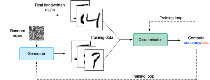
There are many architectures to consider for building the discriminator and the generator. We could build a deep neural network or Convolutional Neural Network (CNN) as well as other options.
TimeGAN
In the context of time series we face not only the problem of matching the features of synthetic and real data sequences, but also calibrating the time dynamics of the underlying generation process. TimeGAN addresses these challenges by using an unsupervised adversarial loss on both real and synthetic sequences, coupled with a stepwise supervised loss using the original data as supervision, thereby explicitly encouraging the model to capture the stepwise conditional distributions in the data. This takes advantage of the fact that there is more information in the training data than simply whether each datum is real or synthetic; we can expressly learn from the transition dynamics from real sequences.
A further innovative feature of the TimeGAN model in the introduction of an embedding network to provide a reversible mapping between features and latent representations, thereby reducing the high-dimensionality of the adversarial learning space. This capitalizes on the fact the temporal dynamics of even complex systems are often driven by fewer and lower-dimensional factors of variation.
Importantly, the supervised loss is minimized by jointly training both the embedding and generator networks, such that the latent space not only serves to promote parameter efficiency—it is specifically conditioned to facilitate the generator in learning temporal relationships.
The figure below shows how the various components are arranged and how the information flows between them during training in TimeGAN.
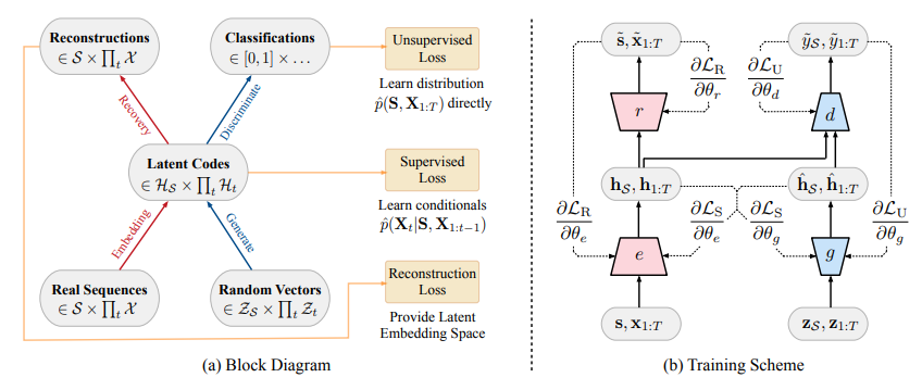
Further details of the TimeGAN model can be found in the paper and in the accompanying GitHub repository, which is found here.
Evaluating the Performance of TimeGAN
The researchers test the TimeGAN methodology using several different datasets, such as daily stock data for the period 2004 to 2019 downloaded from Google, including as features the volume and high, low, opening, and closing prices.
The TimeGAN model is trained for 50,000 epochs with a batch size of 128, using a 24-period rolling window, which the authors found to be the optimal window size. The trained synthesizer produces samples comprising a (128 x 24 x 5) dataframe of price and volume data which can then be compared to the original stock series. It is worth noting that the starting prices of each 24-period window are generated independently, meaning that, for example, the opening price in one sample window might be 10x larger than in another window. This immediately indicates one of the drawbacks of the TimeGAN approach: i.e. that the window length of the generated data is fixed and it can be challenging to stitch windows together to create a longer synthetic series, given that the initial prices for each vary considerably from window to window.
The data visualization methods chosen by the authors to evaluate the performance of the synthetic series in reproducing the features of the original series is problematic, at least as far as stock data is concerned. Both TSNE and PCA plots of the real vs. synthetic data appear to indicate a very close match:
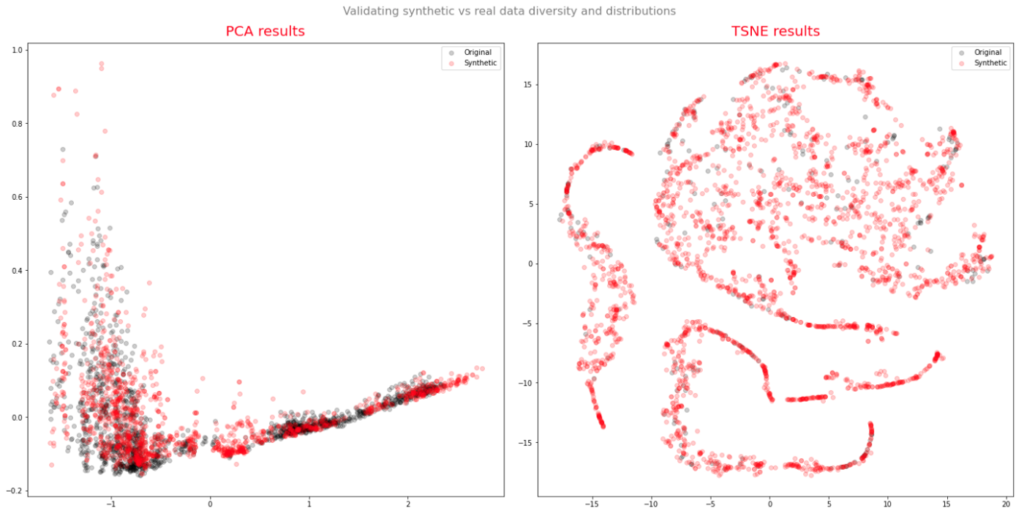
This illustrates how misleading it can be to rely on data visualization for inference purposes. For stock data, there are some very basic tests that should first be performed to ensure the consistency of the synthetic output. In particular, in each row of the window, the High should exceed the Open, Low and Close prices, with the Low price falling below the Open, High and Close prices.
In my experimentation I found that after training the model for 50,000 epochs, the synthetic data failed these basic tests in around 15% of the sample. Further training rounds up to 100,000 epochs reduced the error rate to only 5% and it should be possible to eliminate almost all of these basic data issues with further rounds of training.
However, another basic problem with the synthetic data rapidly becomes apparent: the period to period (in this case, daily) returns have a strong tendency to diminish over time, typically being an order of magnitude larger at the start of each window than towards the end. This pattern of behavior is bound to introduce spurious autocorrelation and volatility-decay effects that are nowhere to be found in the real data series.
Finally, the fixed, limited window size and the independence of each window sample of synthetic data make it impossible to account for important characteristics such as volatility clustering or long memory effects in any adequate way.
Taken together, these flaws render the synthetic stock data produced by TimeGAN significantly unrepresentative and highly unreliable for modelling purposes.
Conclusion
TimeGAN is an important innovation in the field of synthetic data generation, with particular relevance to time series data. However it has significant limitations that make its application to financial time series problematic, in regard to the fixed window length, inconsistencies in the price data and spurious autocorrelation in the returns of the synthetic series it generates.