Backtest vs. Trading Reality

Kris Sidial, whose Twitter posts are often interesting, recently posted about the reality of trading profitability vs backtest performance, as follows:

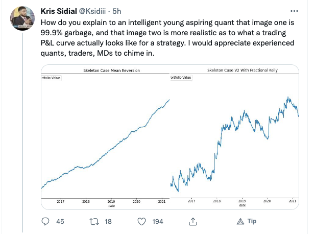
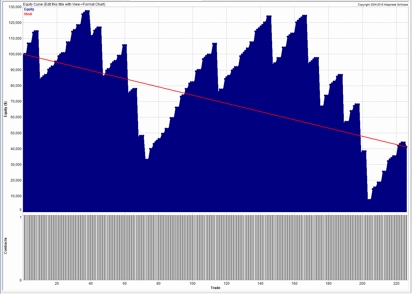
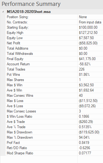
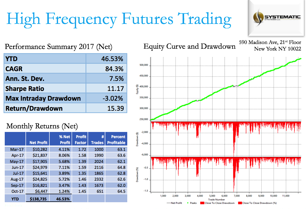
While I certainly agree that the latter example is more representative of a typical trader’s P&L, I don’t concur that the first P&L curve is necessarily “99.9% garbage”. There are many strategies that have equity curves that are smoother and more monotonic than those of Kris’s Skeleton Case V2 strategy. Admittedly, most of these lie in the area of high frequency, which is not Kris’s domain expertise. But there are also lower frequency strategies that produce results which are not dissimilar to those shown the first chart.

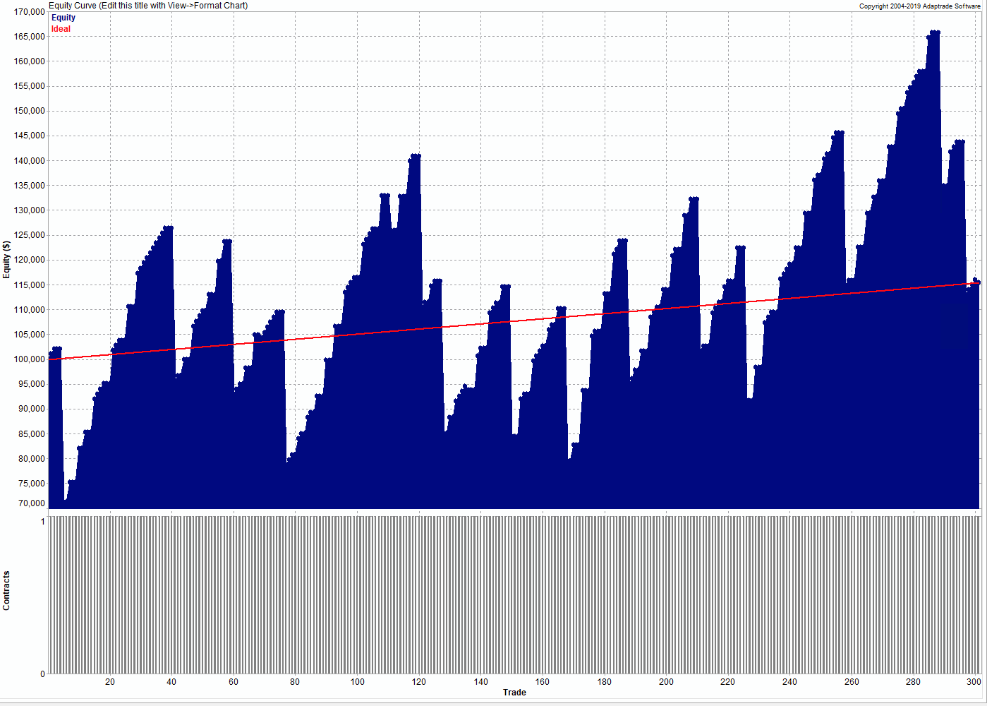
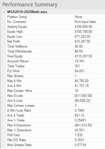
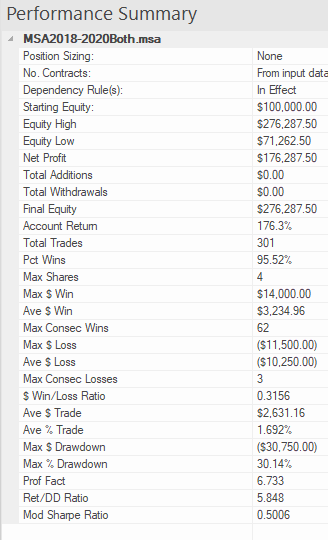
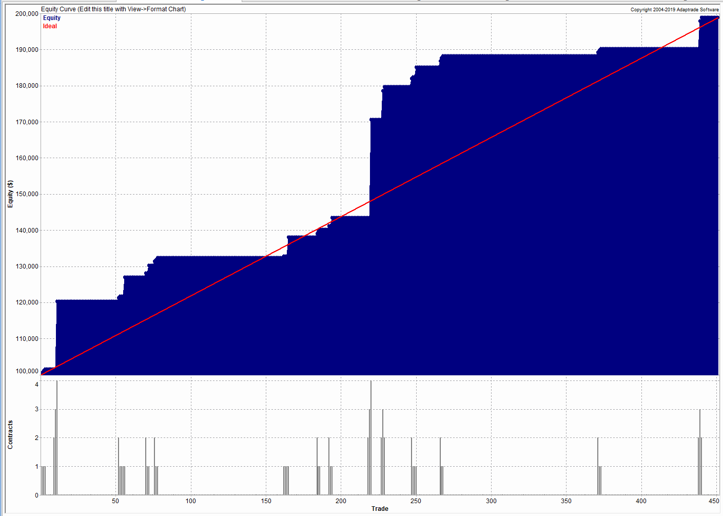
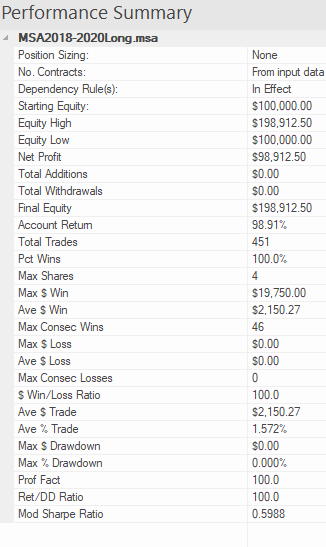
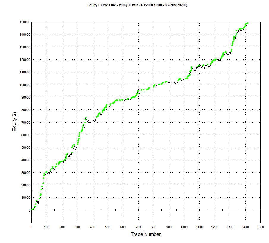
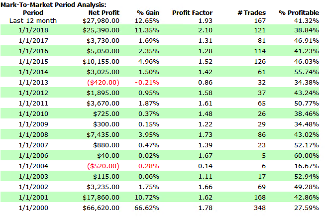
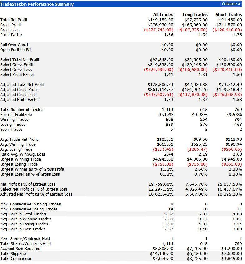
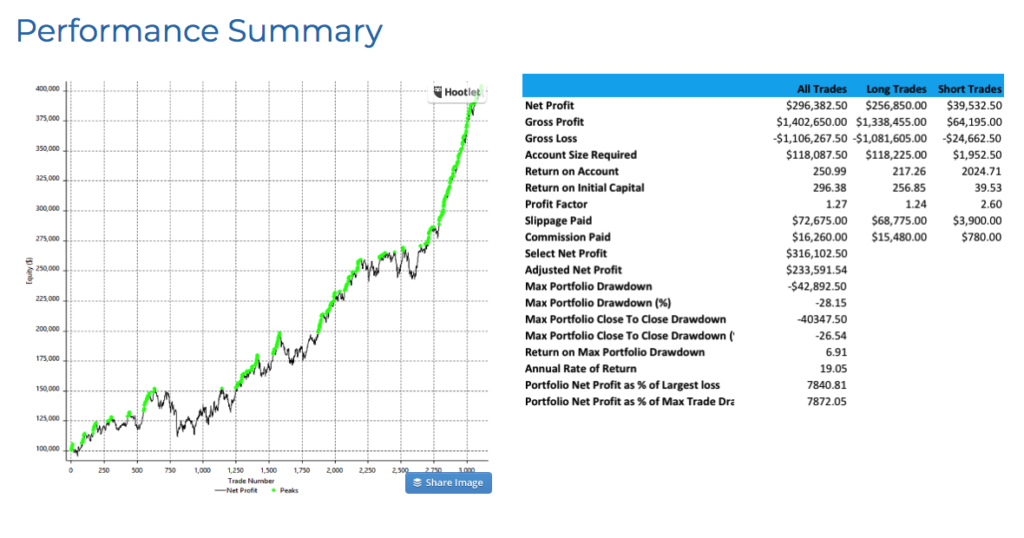
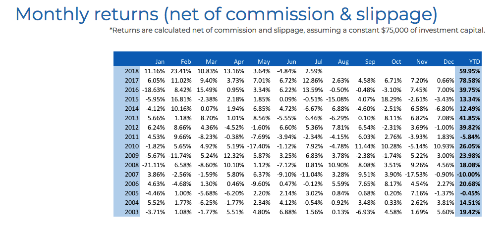
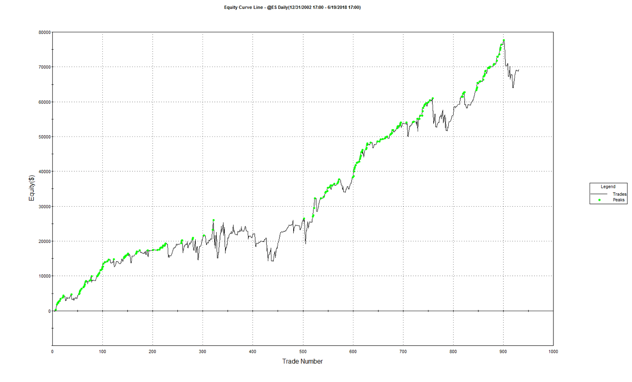
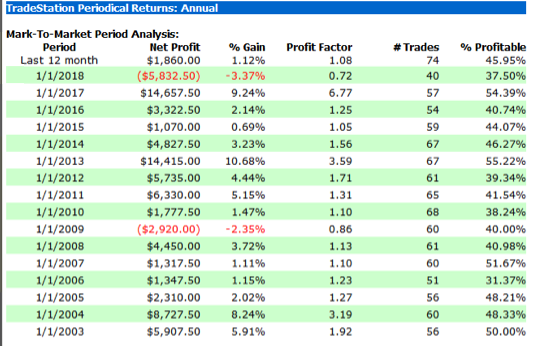
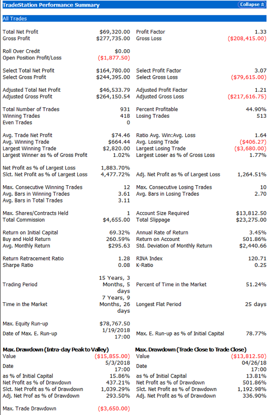
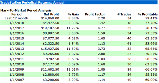
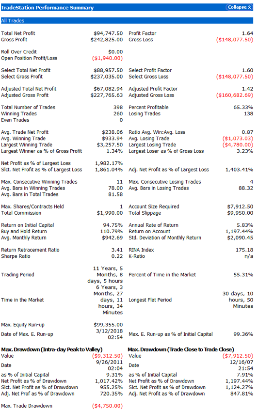
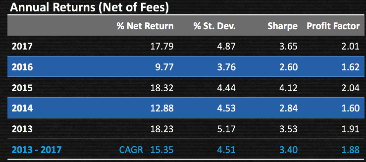
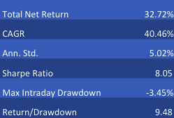
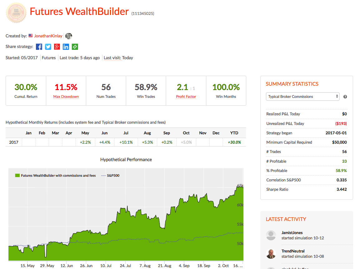
As a case in point, consider the following strategy for the S&P 500 E-Mini futures contract, described in more detail below. The strategy was developed using 15-minute bar data from 1999 to 2012, and traded live thereafter. The live and backtest performance characteristics are almost indistinguishable, not only in terms of rate of profit, but also in regard to strategy characteristics such as the no. of trades, % win rate and profit factor.

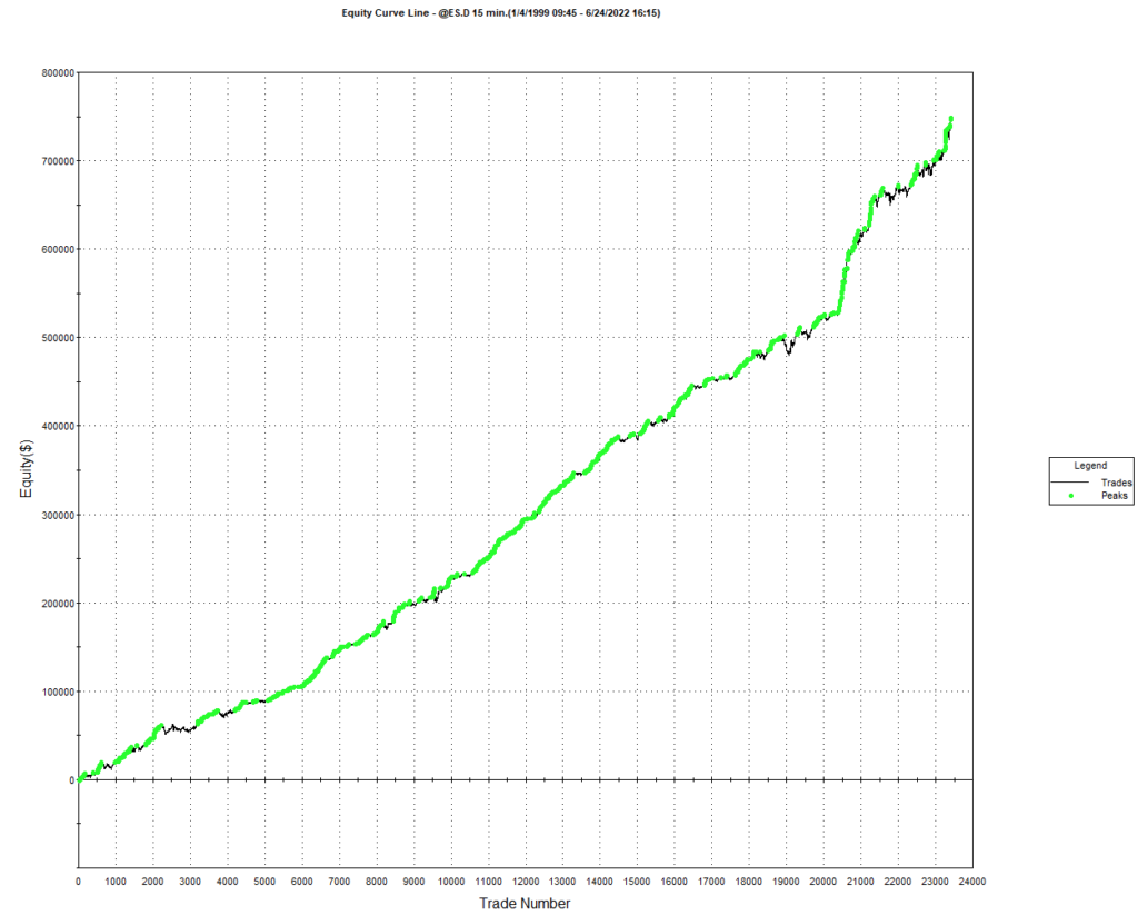
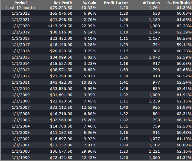
Just in case you think the picture is a little too rosy, I would point out that the average profit factor is 1.25, which means that the strategy is generating only 25% more in profits than losses. There will be big losing trades from time to time and long sequences of losses during which the strategy appears to have broken down. It takes discipline to resist the temptation to “fix” the strategy during extended drawdowns and instead rely on reversion to the mean rate of performance over the long haul. One source of comfort to the trader through such periods is that the 60% win rate means that the majority of trades are profitable.

As you read through the replies to Kris’s post, you will see that several of his readers make the point that strategies with highly attractive equity curves and performance characteristics are typically capital constrained. This is true in the case of this strategy, which I trade with a very modest amount of (my own) capital. Even trading one-lots in the E-Mini futures I occasionally experience missed trades, either on entry or exit, due to limit orders not being filled at the high or low of a bar. In scaling the strategy up to something more meaningful such as a 10-lot, there would be multiple partial fills to deal with. But I think it would be a mistake to abandon a high performing strategy such as this just because of an apparent capacity constraint. There are several approaches one can explore to address the issue, which may be enough to make the strategy scalable.

Where (as here) the issue of scalability relates to the strategy fill rate on limit orders, a good starting point is to compute the extreme hit rate, which is the proportion of trades that take place at the high or low of the bar. As a rule of thumb, for strategies running on typical low frequency infrastructure an extreme hit rate of 10% or less is manageable; anything above that level quickly becomes problematic. If the extreme hit rate is very high, e.g. 25% or more, then you are going to have to pay a great deal of attention to the issues of latency and order priority to make the strategy viable in practise. Ultimately, for a high frequency market making strategy, most orders are filled at the extreme of each “bar”, so almost all of the focus in on minimizing latency and maintaining a high queue priority, with all of the attendant concerns regarding trading hardware, software and infrastructure.

Next, you need a strategy for handling missed trades. You could, for example, decide to skip any entry trades that are missed, while manually entering unfilled exit trades at the market. Or you could post market orders for both entry and exit trades if they are not filled. An extreme solution would be to substitute market-if-touched orders for limit orders in your strategy code. But this would affect all orders generated by the system, not just the 10% at the high or low of the bar and is likely to have a very adverse affect on overall profitability, especially if the average trade is low (because you are paying an extra tick on entry and exit of every trade).

The above suggests that you are monitoring the strategy manually, running simulation and live versions side by side, so that you can pick up any trades that the strategy should have taken, but which have been missed. This may be practical for a strategy that trades during regular market hours, but not for one that also trades the overnight session.

An alternative approach, one that is commonly applied by systematic traders, is to automate the handling of missed trades. Typically the trader will set a parameter that converts a limit order to a market order X seconds after a limit price has been traded but not filled. Of course, this will result in paying up an extra tick (or more) to enter trades that perhaps would have been filled if one had waited longer than X seconds. It will have some negative impact on strategy profitability, but not too much if the extreme hit rate is low. I tend to use this method for exit trades, preferring to skip any entry trades that don’t get filled at the limit price.

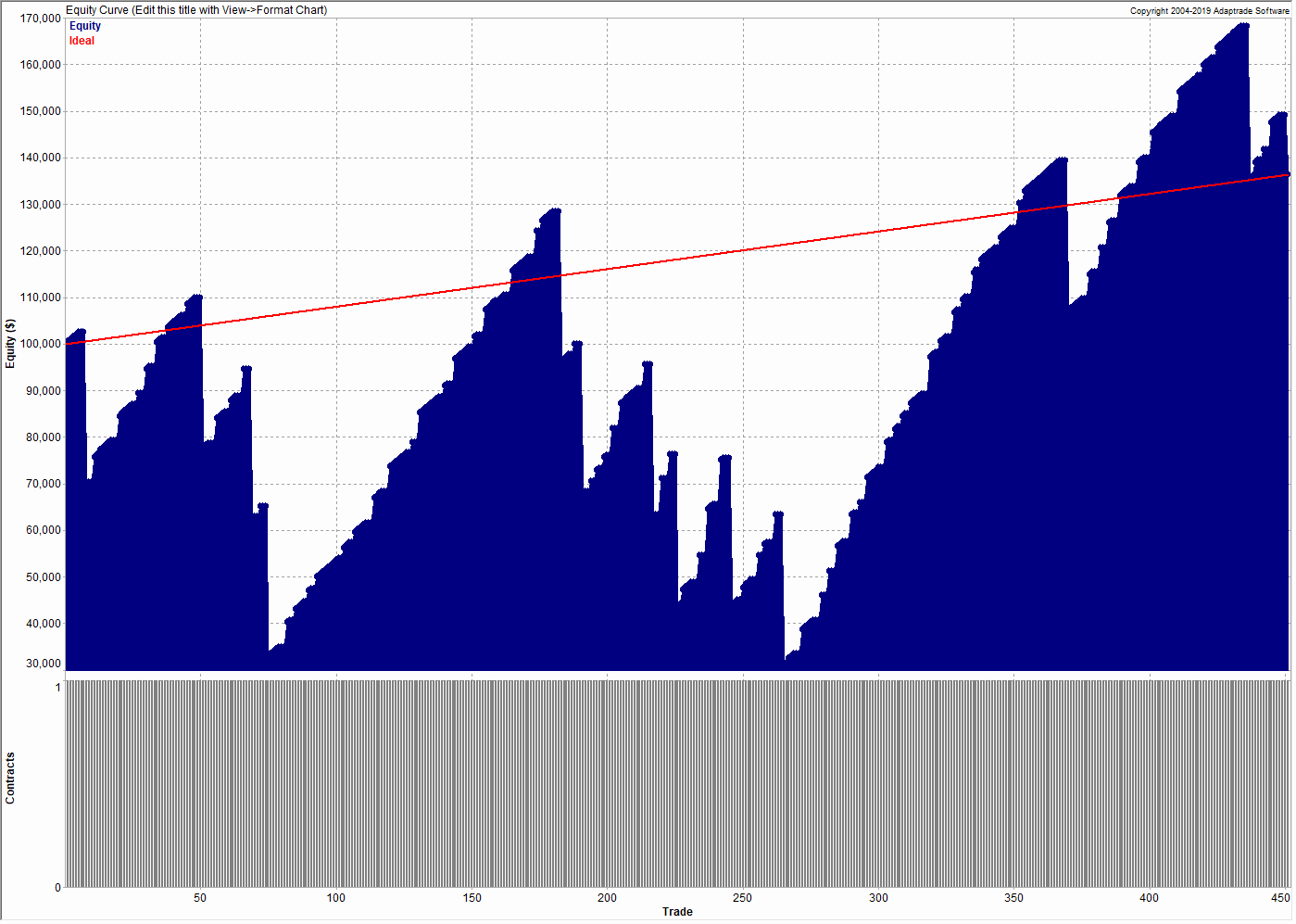
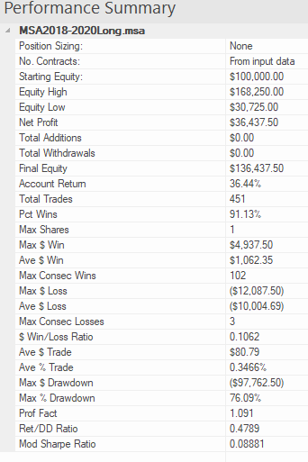
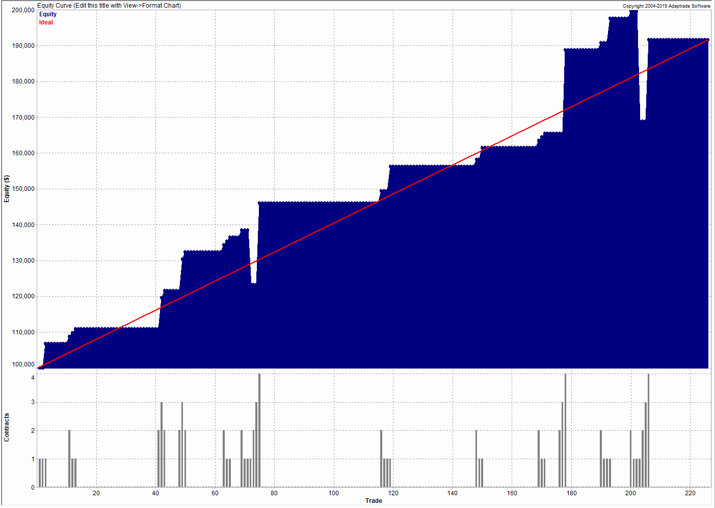
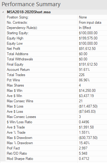
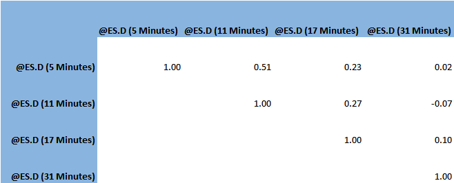
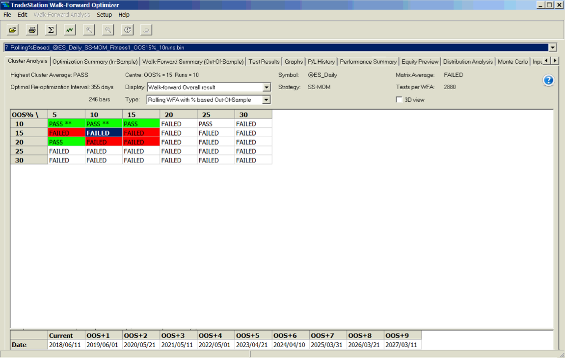
Beyond these simple measures, there are several other ways to extend the capacity of the strategy. An obvious place to start is by evaluating strategy performance on different session times and bar lengths. So, in this case, we might look at deploying the strategy on both the day and night sessions. We can also evaluate performance on bars of different length. This will give different entry and exit points for individual trades and trades that are at the extreme of a bar on one timeframe may not be at the high or low of a bar on the other timescale. For example, here is the (simulated) performance of the strategy on 13 minute bars:

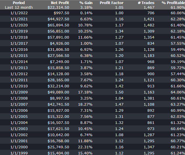
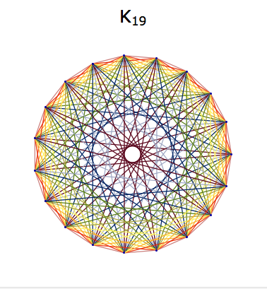
There is a reason for choosing a bar interval such as 13 minutes, rather than the more commonplace 5- or 10 minutes, as explained in this post:

Trading Prime Market Cycles

Finally, it is worth exploring whether the strategy can be applied to other related markets such as NQ futures, for example. Typically this will entail some change to the strategy code to reflect the difference in price levels, but the thrust of the strategy logic will be similar. Another approach is to use the signals from the current strategy as inputs – i.e. alpha generators – for a derivative strategy, such as trading the SPY ETF based on signals from the ES strategy. The performance of the derived strategy may not be as good, but in a product like SPY the capacity might be larger.

November 15, 2021November 15, 2021

Hedged Cryptocurrency Strategies

Hedged-BTC-v2

October 7, 2020

A Meta-Strategy in S&P 500 E-Mini Futures

In earlier posts I have described the idea of a meta-strategy as a strategies that trades strategies. It is an algorithm, or set of rules, that is used to decide when to trade an underlying strategy. In some cases a meta-strategy may influence the size in which the underlying strategy is traded, or may even amend the base code. In other word, a meta-strategy actively “trades” an underlying strategy, or group of strategies, much as in the same way a regular strategy may actively trade stocks, going long or short from time to time. One distinction is that a meta-strategy will rarely, if ever, actually “short” an underlying strategy – at most it will simply turn the strategy off (reduce the position size to zero) for a period.

For a more detailed description, see this post:

Improving Trading System Performance Using a Meta-Strategy

In this post I look at a meta-strategy that developed for a client’s strategy in S&P E-Mini futures. What is extraordinary is that the underlying strategy was so badly designed (not by me!) and performs so poorly that no rational systematic trader would likely give it a second look – instead he would toss it into the large heap of failed ideas that all quantitative researchers accumulate over the course of their careers. So this is a textbook example that illustrates the power of meta-strategies to improve, or in this case transform, the performance of an underlying strategy.

1. The Strategy

The Target Trader Strategy (“TTS”) is a futures strategy applied to S&P 500 E-Mini futures that produces a very high win rate, but which occasionally experiences very large losses. The purpose of the analysis if to find methods that will:

1) Decrease the max loss / drawdown
2) Increase the win rate / profitability

For longs the standard setting is entry 40 ticks below the target, stop loss 1000 ticks below the target, and then 2 re-entries 100 ticks below entry 1 and 100 ticks below entry 2

For shorts the standard is entry 80 ticks above the target. stop loss 1000 ticks above the target, and then 2 re-entries 100 ticks above entry 1 and 100 ticks above entry 2

For both directions its 80 ticks above/below for entry 1, 1000 tick stop, and then 1 re entry 100 ticks above/below, and then re-entry 2 100 ticks above/below entry 2

2. Strategy Performance

2.1 Overall Performance

The overall performance of the strategy over the period from 2018 to 2020 is summarized in the chart of the strategy equity curve and table of performance statistics below.
These confirm that, while the win rate if very high (over 84%) there strategy experiences many significant drawdowns, including a drawdown of -$61,412.50 (-43.58%). The total return is of the order of 5% per year, the strategy profit factor is fractionally above 1 and the Sharpe Ratio is negligibly small. Many traders would consider the performance to be highly unattractive.

2.2 Long Trades

We break the strategy performance down into long and short trades, and consider them separately. On the long side, the strategy has been profitable, producing a gain of over 36% during the period 2018-2020. It also suffered catastrophic drawdown of over -$97,000 during that period:

2.3 Short Trades

On the short side, the story is even worse, producing an overall loss of nearly -$59,000:

3. Improving Strategy Performance with a Meta-Strategy

We considered two possible methods to improve strategy performance. The first method attempts to apply technical indicators and other data series to improve trading performance. Here we evaluated price series such as the VIX index and a wide selection of technical indicators, including RSI, ADX, Moving Averages, MACD, ATR and others. However, any improvement in strategy performance proved to be temporary in nature and highly variable, in many cases amplifying the problems with the strategy performance rather than improving them.

The second approach proved much more effective, however. In this method we create a meta-strategy which effectively “trades the strategy”, turning it on and off depending on its recent performance. The meta-strategy consists of a set of rules that determines whether or not to continue trading the strategy after a series of wins or losses. In some cases the meta-strategy may increase the trade size for a sequence of trades, at times when it considers the conditions for the underlying strategy to be favorable.

The result of applying the meta-strategy are described in the following sections.

3.1 Long & Short Strategies with Meta-Strategy Overlay

The performance of the long/short strategies combined with the meta-strategy overlay are set out in the chart and table below.
The overall improvements can be summarized as follows:

Net profit increases from $15,387 to $176,287
Account return rises from 15% to 176%
Percentage win rate rises from 84% to 95%
Profit factor increases from 1.0 to 6.7
Average trade rises from $51 to $2,631
Max $ Drawdown falls from -$61,412 to -$30,750
Return/Max Drawdown ratio rises from 0.35 to 5.85
The modified Sharpe ratio increases from 0.07 to 0.5

Taken together, these are dramatic improvements to every important aspect of strategy performance.

There are two key rules in the meta-strategy, applicable to winning and losing trades:

Rule for winning trades:
After 3 wins in a row, skip the next trade.

Rule for losing trades:
After 3 losses in a row, add 1 contract until the first win. Subtract 1 contract after each win until the next loss, or back to 1 contract.

3.2 Long Trades with Meta-Strategy

The meta-strategy rules produce significant improvements in the performance of both the long and short components of the strategy. On the long side the percentage win rate is increased to 100% and the max % drawdown is reduced to 0%:

3.3 Short Trades with Meta-Strategy

Improvements to the strategy on the short side are even more significant, transforming a loss of -$59,000 into a profit of $91,600:

4. Conclusion

A meta-strategy is a simple, yet powerful technique that can transform the performance of an underlying strategy. The rules are often simple, although they can be challenging to implement. Meta strategies can be applied to almost any underlying strategy, whether in futures, equities, or forex. Worthwhile improvements in strategy performance are often achievable, although not often as spectacular as in this case.

If any reader is interested in designing a meta-strategy for their own use, please get in contact.

August 4, 2020

Daytrading Index Futures Arbitrage

Trading with Indices

I have always been an advocate of incorporating index data into one’s trading strategies. Since they are not tradable, the “market” in index products if often highly inefficient and displays easily identifiable patterns that can be exploited by a trader, or a trading system. In fact, it is almost trivially easy to design “profitable” index trading systems and I gave a couple of examples in the post below, including a system producing stellar results in the S&P 500 Index.

http://jonathankinlay.com/2016/05/trading-with-indices/

Of course such systems are not directly useful. But traders often use signals from such a system as a filter for an actual trading system. So, for example, one might look for a correlated signal in the S&P 500 index as a means of filtering trades in the E-Mini futures market or theSPDR S&P 500 ETF (SPY).

Multi-Strategy Trading Systems

This is often as far as traders will take the idea, since it quickly gets a lot more complicated and challenging to build signals generated from an index series into the logic of a strategy designed for related, tradable market. And for that reason, there is a great deal of unexplored potential in using index data in this way. So, for instance, in the post below I discuss a swing trading system in the S&P500 E-mini futures (ticker: ES) that comprises several sub-systems build on prime-valued time intervals. This has the benefit of minimizing the overlap between signals from multiple sub-systems, thereby increasing temporal diversification.

http://jonathankinlay.com/2018/07/trading-prime-market-cycles/

A critical point about this system is that each of sub-systems trades the futures market based on data from both the E-mini contract and the S&P 500 cash index. A signal is generated when the system finds particular types of discrepancy between the cash index and corresponding futures, in a quasi risk-arbitrage.

Arbing the NASDAQ 100 Index Futures

Developing trading systems for the S&P500 E-mini futures market is not that hard. A much tougher challenge, at least in my experience, is presented by the E-mini NASDAQ-100 futures (ticker: NQ). This is partly to do with the much smaller tick size and different market microstructure of the NASDAQ futures market. Additionally, the upward drift in equity related products typically favors strategies that are long-only. Where a system trades both long and short sides of the market, the performance on the latter is usually much inferior. This can mean that the strategy performs poorly in bear markets such as 2008/09 and, for the tech sector especially, the crash of 2000/2001. Our goal was to develop a daytrading system that might trade 1-2 times a week, and which would perform as well or better on short trades as on the long side. This is where NASDAQ 100 index data proved to be especially helpful. We found that discrepancies between the cash index and futures market gave particularly powerful signals when markets seemed likely to decline. Using this we were able to create a system that performed exceptionally well during the most challenging market conditions. It is notable that, in the performance results below (for a single futures contract, net of commissions and slippage), short trades contributed the greater proportion of total profits, with a higher overall profit factor and average trade size.

Conclusion: Using Index Data, Or Other Correlated Signals, Often Improves Performance

It is well worthwhile investigating how non-tradable index data can be used in a trading strategy, either as a qualifying signal or, more directly, within the logic of the algorithm itself. The greater challenge of building such systems means that there are opportunities to be found, even in well-mined areas like index futures markets. A parallel idea that likewise offers plentiful opportunity is in designing systems that make use of data on multiple time frames, and in correlated markets, for instance in the energy sector.Here one can identify situations in which, under certain conditions, one market has a tendency to lead another, a phenomenon referred to as Granger Causality.

July 7, 2020July 7, 2020

Trading Prime Market Cycles

Magicicada is the genus of the 13-year and 17-year periodical cicadas of eastern North America. Magicicada species spend most of their 13- and 17-year lives underground feeding on xylem fluids from the roots of deciduous forest trees in the eastern United States. After 13 or 17 years, mature cicada nymphs emerge in the springtime at any given locality, synchronously and in tremendous numbers. Within two months of the original emergence, the lifecycle is complete, the eggs have been laid, and the adult cicadas are gone for another 13 or 17 years.

The emergence period of large prime numbers (13 and 17 years) has been hypothesized to be a predator avoidance strategy adopted to eliminate the possibility of potential predators receiving periodic population boosts by synchronizing their own generations to divisors of the cicada emergence period. If, for example, the cycle length was, say, 12 years, then the species would be exposed to predators regenerating over cycles of 2, 3, 4, or 6 years. Limiting their cycle to a large prime number reduces the variety of predators the species is likely to face.

Prime Cycles in Trading Strategies

What has any of this to do with trading? When building a strategy in a particular market we might start by creating a model that works reasonably well on, say, 5-minute bars. Then, in order to improve the risk-adjusted returns we might try create a second sub-strategy on a different frequency. This will hopefully result in a new series of signals, an increase in the number of trades, and corresponding improvement in the risk-adjusted returns of the overall strategy. This phenomenon is referred to as temporal diversification.

What time frequency should we select for our second sub-strategy? There are many factors to consider, of course, but one of them is that we would like to see as few duplicate signals between the two sub-strategies. Otherwise we will simply be replicating trades, rather than reducing the overall level of strategy risk through temporal diversification. The best way to minimize the overlap in signals generated by multiple sub-strategies is to use prime number bar frequencies (5 minute, 7 minute, 11 minute, etc).

S&P500 Swing Trading Strategy

An example of this approach is our EMini Swing Trading strategy which we operate on our Systematic Algotrading Platform. This strategy is actually a combination of several different sub-strategies that operate on 5-minute, 11-minute, 17-minute and 31-minute bars. Each strategy focuses on a different set of characteristics of the S&P 500 futures market, but the key point here is that the trading signals very rarely overlap and indeed several of the sub-strategies have a low correlation.

The resulting increase in trade frequency and temporal diversification produces very attractive risk-adjusted performance: after an exceptional year in 2017 which saw a 78.58% net return, the strategy is already at +60% YTD in 2018 and showing no sign of slowing down.

Investors can auto-trade the E-Mini Swing Trading strategy and many other strategies in their own account – see the Leaderboard for more details.

June 2, 2020

A Simple Momentum Strategy

Momentum trading strategies span a diverse range of trading ideas. Often they will use indicators to determine the recent underlying trend and try to gauge the strength of the trend using measures of the rate of change in the price of the asset.

One very simple momentum concept, a strategy in S&P500 E-Mini futures, is described in the following blog post:

http://www.quantifiedstrategies.com/buy-when-sp-500-makes-new-intraday-high/

The basic idea is to buy the S&P500 E-Mini futures when the contract makes a new intraday high. This is subject to the qualification that the Internal Bar Strength fall below a selected threshold level. In order words, after a period of short-term weakness – indicated by the low reading of the Internal Bar Strength – we buy when the futures recover to make a new intraday high, suggesting continued forward momentum.

IBS is quite a useful trading indicator, which you can learn more about in these posts:

http://jonathankinlay.com/2016/06/the-internal-bar-strength-indicator/

http://jonathankinlay.com/2016/06/quick-note-internal-bar-strength-stationarity/

I have developed a version of the intraday-high strategy, using parameters to generalize it and allow for strategy optimization. The Easylanguage code for my version of the strategy is as follows:

Inputs:
nContracts(1),
ndaysHigh(5),
IBSlag(1),
IBStrigger(0.15);

Vars:

IBS(0.5);

If H[IBSlag] > L[IBSlag] then
Begin
IBS=(H[IBSlag]-C[IBSlag])/(H[IBSlag]-L[IBSlag]);
end;
If (IBS <= IBStrigger) and (H[0] >= Highest(High, ndaysHigh)) then
begin
Buy nContracts contracts this bar on close;
end;

If C[0] > H[1] then
begin
Sell all contracts this bar on close;
end;

The performance results for the strategy appear quite promising, despite the downturn in strategy profitability in 2018 to date (all performance results are net of slippage and commission):

Robustness Testing with Walk Forward Optimization

We evaluate the robustness of the strategy using the Walk Forward Optimization feature in Tradestation. Walk forward analysis is the process of optimizing a trading system using a limited set of parameters, and then testing the best optimized parameter set on out-of-sample data. This process is similar to how a trader would use an automated trading system in real live trading. The in-sample time window is shifted forward by the period covered by the out-of-sample test, and the process is repeated. At the end of the test, all of the recorded results are used to assess the trading strategy.

In other words, walk forward analysis does optimization on a training set; tests on a period after the set and then rolls it all forward and repeats the process. This gives a larger out-of-sample period and allows the system developer to see how stable the system is over time.

The image below illustrates the walk forward analysis procedure. An optimization is performed over a longer period (the in-sample data), and then the optimized parameter set is tested over a subsequent shorter period (the out-of-sample data). The optimization and testing periods are shifted forward, and the process is repeated until a suitable sample size is achieved.

Tradestation enables the user to run a battery of WFO tests, using different size in-sample and out-of-sample sizes and number of runs. The outcome of each test is evaluated on several specific criteria such as the net profit and drawdown and only if the system meets all of the criteria is the test designated as a “Pass”. This gives the analyst a clear sense of the robustness of his strategy across multiple periods and sample sizes.

A WFO cluster analysis summary for the momentum strategy is illustrated below. The cluster test is designated as “Failed” overall, since the strategy failed to meet the test criteria for a preponderance of the individual walk-forward tests. The optimal parameters found in each test vary considerably over the sample periods spanning 2003-2018, giving concerns about the robustness of the strategy under changing market conditions.

Improving the Strategy

We can improve both the performance and robustness of our simple momentum strategy by combining it with several other trend and momentum indicators. One such example is illustrated in the performance charts and tables below. The strategy has performed well in both bull and bear markets and in both normal and volatile market conditions:

A WFO cluster analysis indicates that the revised momentum strategy is highly robust to the choice of sample size and strategy parameters, as it passes every test in the 30-cell WFO analysis cluster table:

Conclusion

Momentum strategies are well known and easy to develop using standard methodologies, such as the simple indicators used in this example. They tend to work well in most equity index futures markets, and in some commodity markets too. One of their big drawbacks, however, is that they typically go through periods of poor performance and need to be tested thoroughly for robustness in order to ensure satisfactory results under the full range of market conditions.

May 26, 2020

Finding Alpha in 2018

Given the current macro-economic environment, where should investors focus their search for sources of alpha in the year ahead? By asking enough economists or investment managers you will find as many different opinions on the subject as would care to, no doubt many of them conflicting. These are some thoughts on the subject from my perspective, as a quantitative hedge fund manager.

Global Market Performance in 2017

Let’s begin by reviewing some of the best and worst performing assets of 2017 (I am going to exclude cryptocurrencies from the ensuing discussion). Broadly speaking, the story across the piste has been one of strong appreciation in emerging markets, both in equities and currencies, especially in several of the Eastern European economies. In Government bond markets Greece has been the star of the show, having stepped back from the brink of the economic abyss. Overall, international diversification has been a key to investment success in 2017 and I believe that pattern will hold in 2018.

US Yield Curve and Its Implications

Another key development that investors need to take account of is the extraordinary degree of flattening of the yield curve in US fixed income over the course of 2017:

This process has now likely reached the end point and will begin to reverse as the Fed and other central banks in developed economies start raising rates. In 2018 investors should seek to protect their fixed income portfolios by shortening duration, moving towards the front end of the curve.

US Volatility and Equity Markets

A prominent feature of US markets during 2017 has been the continuing collapse of equity index volatility, specifically the VIX Index, which reached an all-time low of 9.14 in November and continues to languish at less than half the average level of the last decade:

Source: Wolfram Alpha

One consequence of the long term decline in volatility has been to drastically reduce the profitability of derivatives markets, for both traders and market makers. Firms have struggled to keep up with the high cost of technology and the expense of being connected to the fragmented U.S. options market, which is spread across 15 exchanges. Earlier in 2017, Interactive Brokers Group Inc. sold its Timber Hill options market-making unit — a pioneer of electronic trading — to Two Sigma Securities. Then, in November, Goldman Sachs announced it was shuttering its option market making business in US exchanges, citing high costs, sluggish volume and low volatility.

The impact has likewise been felt by volatility strategies, which performed well in 2015 and 2016, only to see returns decline substantially in 2017. Our own Systematic Volatility strategy, for example, finished the year up only 8.08%, having produced over 28% in the prior year.

One side-effect of low levels of index volatility has been a fall in stock return correlations, and, conversely, a rise in the dispersion of stock returns. It turns out that index volatility and stock correlation are themselves correlated and indeed, cointegrated:

http://jonathankinlay.com/2017/08/correlation-cointegration/

In simple terms, stocks have a tendency to disperse more widely around an increasingly sluggish index. The “kinetic energy” of markets has to disperse somewhere and if movements in the index are muted then relative movement in individual equity returns will become more accentuated. This is an environment that ought to favor stock picking and both equity long/short and market neutral strategies should outperform. This certainly proved to be the case for our Quantitative Equity long/short strategy, which produced a net return of 17.79% in 2017, but with an annual volatility of under 5%:

Looking ahead to 2018, I expect index volatility and equity correlations rise as the yield curve begins to steepen, producing better opportunities for volatility strategies. Returns from equity long/short and market neutral strategies may moderate a little as dispersion diminishes.

Futures Markets

Big increases in commodity prices and dispersion levels also lead to improvements in the performance of many CTA strategies in 2017. In the low frequency space our Futures WealthBuilder strategy produced a net return of 13.02% in 2017, with a Sharpe Ratio above 3 (CAGR from inception in 2013 is now at 20.53%, with an average annual standard deviation of 6.36%). The star performer, however, was our High Frequency Futures strategy. Since launch in March 2017 this has produce a net return of 32.72%, with an annual standard deviation of 5.02%, on track to generate an annual Sharpe Ratio above 8 :

Looking ahead, the World Bank has forecast an increase of around 4% in energy prices during 2018, with smaller increases in the price of agricultural products. This is likely to be helpful to many CTA strategies, which will likely see further enhancements in performance over the course of the year. Higher frequency strategies are more dependent on commodity market volatility, which is seen more likely to rise than fall in the year ahead.

Conclusion

US fixed income investors are likely to want to shorten duration as the yield curve begins to steepen in 2018, bringing with it higher levels of index volatility that will favor equity high frequency and volatility strategies. As in 2017, there is likely much benefit to be gained in diversifying across international equity and currency markets. Strengthening energy prices are likely to sustain higher rates of return in futures strategies during the coming year.

May 19, 2020

Trading Bitcoin

At Systematic Strategies we have developed a brilliant, new investment strategy. We call it buying Bitcoin. It works like this: you take some of your hard-earned fiat and use it to buy Bitcoin. Then, a week or two later, you do the same thing all over again. So far the strategy is up around 400% YTD. Genius.

It’s such a successful strategy that we are tempted to clone it. Buying Litecoin, or Ethereum, spring to mind.

As freshly-minted, bona-fide cryptocurrency entrepreneurs, it is perhaps timely to ponder the roots of this success story and share our discoveries with other, perhaps more rational investors, who may be inclined to treat the whole cryptocurrency malarky as a tulip-Ponzi scheme. First, there is a back-story to this. During the mid 1990’s I was teaching computational finance at Carnegie Mellon to some very bright students who were, naturally enough, playing the market on the side. This was the time of the internet boom with tech stocks like Amazon, Ebay, Sun Microsystems, et al, leading the charge to ever higher levels in the market. The multiples that some of these stocks were trading at were truly astonishing. I had seen something similar just before the crash in the Japanese market towards the end of the 1980’s, when stocks were trading at three-figure multiples. So by around 1997/98 I was becoming increasingly nervous that the tech boom might be at the point of imminent collapse. I conveyed these sentiments to my students, expressing concern that they should not over-commit themselves to what might turn out to be a bubble. My advice was roundly ignored and for the next couple of years I suffered the almost daily humiliation of watching the market indices reach even higher levels, to the joy of dot com investors. When the crash came many lost most, if not all, of their investment. It was like a funeral in the Hamptons that summer. Teary-eyed students asked me for advice as to what they should do to salvage what was left of their investment nest egg. I didn’t have the stomach for gloating. The only piece of advice I could think to offer them was: “learn”. I hope they did. Because here we are again.

What concerned me back in ’98 was not that I didn’t understand the importance of the new internet paradigm: on the contrary, I was an early adopter of the new technologies. I fully understood the potential benefits that a digital business like Amazon enjoyed versus bricks and mortar rivals. But it’s also the case that I under-estimated the potential of a company like Amazon, in several important ways. For instance, I did not foresee how useful and important customer reviews would become (facilitated by the digital medium); nor did I anticipate Amazon being as successful as it has been in broadening the scope of its services from books (then) to just about everything (now); and I also under-estimated the challenge that the new entrants would pose to traditional rivals, who struggled (and often failed) to adapt their hitherto successful business strategies. In other words, my concern didn’t stem from a lack of appreciation of the potential of the new tech companies, although I certainly under-estimated that potential in some cases. Rather, my thinking was that it had gone too far, too fast and that the blistering pace of the market melt-up would inevitably slow. I was right, but way too early. It is notoriously difficult to get the timing of the bubble-popping right, even if the call is correct.

Chaotic trading marks new surge in bitcoin price

In one wild 20 minute period, the price of bitcoin soared $2,000 per coin to more than $19,000 only to drop to $15,000 on the Coinbase trading venue. – Financial Times, Dec 8th, 2017

So to Bitcoin, which is undergoing a similar melt-up. Again, the rationale for the popularity of cryptocurrencies is not hard to fathom, given all the central bank shenanigans of the last decade and the poor reputation that several major banks have earned as serial manipulators of markets in fiat currency substitutes, like gold, or silver. Once again, it appears to me, the entities whose well established business models are most threatened by the arrival of cryptocurrencies have been slow on the uptake and most, like JP Morgan, for instance, are still in denial. The chief threat from cryptocurrencies lies in their potential to dis-intermediate the banks, by allowing users to transact directly with one another, and also Governments, who stand to lose considerable sums in tax revenue. No doubt they will eventually wake up to the scale of threat that Bitcoin poses and respond accordingly in due course – i.e. expect an avalanche of new regulation and government propaganda seeking to equate ownership of Bitcoin with “money laundering”, whatever that preposterous phrase might actually mean. I am not convinced that the genie can be stuffed back into the bottle so easily.

Given the value and scale of the market that cryptocurrencies are in the process of disrupting, i.e. global banking and taxation, the upside potential is indeed enormous. I fully expect the surge to continue for some time. But we can expect a great deal of volatility and several corrections of 20%, or more, along the way. The first of these might arrive next week, as Bitcoin futures start trading, enabling speculators to initiate short positions against the cryptocurrency. Other adverse events are likely to include increased scrutiny by government agencies like the IRS and market regulators like the SEC, although it remains to be seen how effectively they are able to operate in this sphere.

So, with all that said, here are some thoughts on how to play the market, if you must:

Check out this useful Beginner’s Guide to Trading Bitcoin
Invest no more than 10% to 20% of your net worth. Losing this will hurt, but not kill you. Yes, you probably won’t become a Bitcoin billionaire, but neither will you end up in the poor house. Do not, under any circumstances, sell all your assets and plunge in. If you lose your home and the college fund, your wife and kids will never forgive you.
Wait to see if we get a decent pullback after futures trading starts before you buy (more). If that doesn’t happen, it’s up to you to decide whether you want to wait it out or get aboard the train immediately. There is no right answer. At some point you are going to lose at least 20% of the value of your investment. It could be on day one, or six months from now. There is no way to know.
I have read a few articles by traders threatening to short the heck out of the futures market as soon as it opens. For some of them this appears to be revenge for having missed a golden opportunity to buy Bitcoin when it was worth a fraction of the price it trades at today. Please don’t do this. It will be like trying to stop a freight train with your hand. You might get lucky, once or twice, but sooner or later you are going to get run over. And it will hurt a lot.
If you want to trade the short side, or trade the long side more conservatively, consider a pairs trade. By this I mean, for instance, if you do decide to sell Bitcoin futures, consider hedging the position by buying another cryptocurrency like Ethereum or Litecoin. For a detailed description of how to approach this in a more sophisticated way, see these posts:

http://jonathankinlay.com/2017/03/pairs-trading-copulas/

http://jonathankinlay.com/2015/02/developing-statistical-arbitrage-strategies-using-cointegration/

DISCLAIMER

As always, readers are entirely responsible for making their own investment decisions and for any and all consequences arising from them. The author bears no responsibility for any action or decision taken, or not taken, by any investor pursuant to this or other articles and disclaims any responsibility for investment decisions taken by readers of this blog.

May 12, 2020May 12, 2020

Systematic Futures Trading

In its proprietary trading, Systematic Strategies primary focus in on equity and volatility strategies, both low and high frequency. In futures, the emphasis is on high frequency trading, although we also run one or two lower frequency strategies that have higher capacity, such as the Futures WealthBuilder. The version of WealthBuilder running on the Collective 2 site has performed very well in 2017, with net returns of 30% and a Sharpe Ratio of 3.4:

In the high frequency space, our focus is on strategies with very high Sharpe Ratios and low drawdowns. We trade a range of futures products, including equity, fixed income, metals and energy markets. Despite the current low levels of market volatility, these strategies have performed well in 2017:

Building high frequency strategies with double-digit Sharpe Ratios requires a synergy of computational capability and modeling know-how. The microstructure of futures markets is, of course, substantially different to that of equity or forex markets and the components of the model that include microstructure effects vary widely from one product to another. There can be substantial variations too in the way that time is handled in the model – whether as discrete or continuous “wall time”, in trade time, or some other measure. But some of the simple technical indicators we use – moving averages, for example – are common to many models across different products and markets. Machine learning plays a role in most of our trading strategies, including high frequency.

Here are some relevant blog posts that you may find interesting:

http://jonathankinlay.com/2016/04/high-frequency-trading-equities-vs-futures/

http://jonathankinlay.com/2015/05/designing-scalable-futures-strategy/

http://jonathankinlay.com/2014/10/day-trading-system-in-vix-futures/

April 21, 2020

The Story of a HFT Strategy

VIX HFT Scalper