Regime-Switching & Market State Modeling

The Excel workbook referred to in this post can be downloaded here.

Market state models are amongst the most useful analytical techniques that can be helpful in developing alpha-signal generators.  That term covers a great deal of ground, with ideas drawn from statistics, econometrics, physics and bioinformatics.  The purpose of this short note is to provide an introduction to some of the key ideas and suggest ways in which they might usefully applied in the context of researching and developing trading systems.

Although they come from different origins, the concepts presented here share common foundational principles:

  1. Markets operate in different states that may be characterized by various measures (volatility, correlation, microstructure, etc);
  2. Alpha signals can be generated more effectively by developing models that are adapted to take account of different market regimes;
  3. Alpha signals may be combined together effectively by taking account of the various states that a market may be in.

Market state models have shown great promise is a variety of applications within the field of applied econometrics in finance, not only for price and market direction forecasting, but also basis trading, index arbitrage, statistical arbitrage, portfolio construction, capital allocation and risk management.

REGIME SWITCHING MODELS

These are econometric models which seek to use statistical techniques to characterize market states in terms of different estimates of the parameters of some underlying linear model.  This is accompanied by a transition matrix which estimates the probability of moving from one state to another.

To illustrate this approach I have constructed a simple example, given in the accompanying Excel workbook.  In this model the market operates as follows:

econometric Where

Yt is a variable of interest (e.g. the return in an asset over the next period t) 

et is an error process with constant variance s2 

S is the market state, with two regimes (S=1 or S=2) 

a0 is the drift in the asset process 

a1 is an autoregressive term, by which the return in the current period is dependent on the prior period return 

b1 is a moving average term, which smoothes the error process 

 This is one of the simplest possible structures, which in more general form can include multiple states, and independent regressions Xi as explanatory variables (such as book pressure, order flow, etc):

econometric


SSALGOTRADING AD

The form of the error process et may also be dependent on the market state.  It may simply be that, as in this example, the standard deviation of the error process changes from state to state.  But the changes can also be much more complex:  for instance, the error process may be non-Gaussian, or it may follow a formulation from the GARCH framework.

In this example the state parameters are as follows:

Reg1 Reg 2
s 0.01 0.02
a0 0.005 -0.015
a1 0.40 0.70
b1 0.10 0.20

What this means is that, in the first state the market tends to trend upwards with relatively low volatility.  In the second state, not only is market volatility much higher, but also the trend is 3x as large in the negative direction.

I have specified the following state transition matrix:

Reg1 Reg2
Reg1 0.85 0.15
Reg2 0.90 0.10

This is interpreted as follows:  if the market is in State 1, it will tend to remain in that state 85% of the time, transitioning to State 2 15% of the time.  Once in State 2, the market tends to revert to State 1 very quickly, with 90% probability.  So the system is in State 1 most of the time, trending slowly upwards with low volatility and occasionally flipping into an aggressively downward trending phase with much higher volatility.

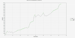
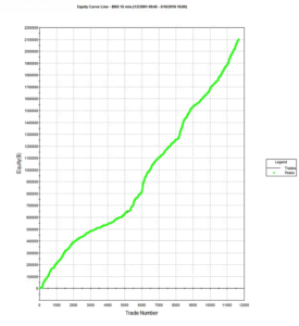
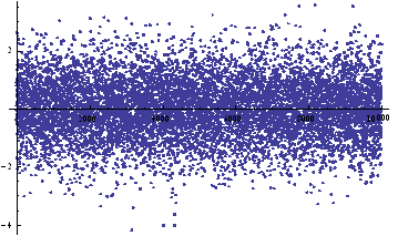
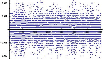
The Generate sheet in the Excel workbook shows how observations are generated from this process, from which we select a single instance of 3,000 observations, shown in sheet named Sample.

The sample looks like this:


Market state 


 As anticipated, the market is in State 1 most of the time, occasionally flipping into State 2 for brief periods.

Market state 

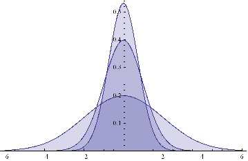
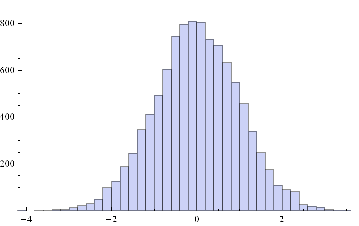
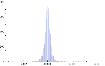
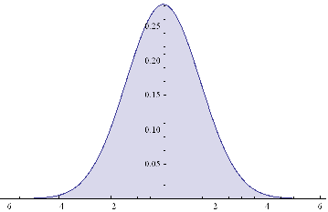
 It is well-known that in financial markets we are typically dealing with highly non-Gaussian distributions.  Non-Normality can arise for a number of reasons, including changes in regimes, as illustrated here.  It is worth noting that, even though in this example the process in either market state follows a Gaussian distribution, the combined process is distinctly non-Gaussian in form, having (extremely) fat tails, as shown by the QQ-plot below.


 Market state

If we attempt to fit a standard ARMA model to the process, the outcome is very disappointing in terms of the model’s poor explanatory power (R2 0.5%) and lack of fit in the squared-residuals:


ARIMA(1,0,1)

         Estimate  Std. Err.   t Ratio  p-Value

Intercept                      0.00037    0.00032     1.164    0.244

AR1                            0.57261     0.1697     3.374    0.001

MA1                           -0.63292    0.16163    -3.916        0

Error Variance^(1/2)           0.02015     0.0004    ——   ——

                       Log Likelihood = 7451.96

                    Schwarz Criterion = 7435.95

               Hannan-Quinn Criterion = 7443.64

                     Akaike Criterion = 7447.96

                       Sum of Squares =  1.2172

                            R-Squared =  0.0054

                        R-Bar-Squared =  0.0044

                          Residual SD =  0.0202

                    Residual Skewness = -2.1345

                    Residual Kurtosis =  5.7279

                     Jarque-Bera Test = 3206.15     {0}

Box-Pierce (residuals):         Q(48) = 59.9785 {0.115}

Box-Pierce (squared residuals): Q(50) = 78.2253 {0.007}

              Durbin Watson Statistic = 2.01392

                    KPSS test of I(0) =  0.2001    {<1} *

                 Lo’s RS test of I(0) =  1.2259  {<0.5} *

Nyblom-Hansen Stability Test:  NH(4)  =  0.5275    {<1}

MA form is 1 + a_1 L +…+ a_q L^q.

Covariance matrix from robust formula.

* KPSS, RS bandwidth = 0.

Parzen HAC kernel with Newey-West plug-in bandwidth.


However, if we keep the same simple form of ARMA(1,1) model, but allow for the possibility of a two-state Markov process, the picture alters dramatically:  now the model is able to account for 98% of the variation in the process, as shown below.


Notice that we have succeeded in estimating the correct underlying transition probabilities, and how the ARMA model parameters change from regime to regime much as they should (small positive drift in one regime, large negative drift in the second, etc).


Markov Transition Probabilities

                    P(.|1)       P(.|2)

P(1|.)            0.080265      0.14613

P(2|.)             0.91973      0.85387


                              Estimate  Std. Err.   t Ratio  p-Value

Logistic, t(1,1)              -2.43875     0.1821    ——   ——

Logistic, t(1,2)              -1.76531     0.0558    ——   ——

Non-switching parameters shown as Regime 1.


Regime 1:

Intercept                     -0.05615    0.00315   -17.826        0

AR1                            0.70864    0.16008     4.427        0

MA1                           -0.67382    0.16787    -4.014        0

Error Variance^(1/2)           0.00244     0.0001    ——   ——


Regime 2:

Intercept                      0.00838     2e-005   419.246        0

AR1                            0.26716    0.08347     3.201    0.001

MA1                           -0.26592    0.08339    -3.189    0.001


                       Log Likelihood = 12593.3

                    Schwarz Criterion = 12557.2

               Hannan-Quinn Criterion = 12574.5

                     Akaike Criterion = 12584.3

                       Sum of Squares =  0.0178

                            R-Squared =  0.9854

                        R-Bar-Squared =  0.9854

                          Residual SD =  0.002

                    Residual Skewness = -0.0483

                    Residual Kurtosis = 13.8765

                     Jarque-Bera Test = 14778.5     {0}

Box-Pierce (residuals):         Q(48) = 379.511     {0}

Box-Pierce (squared residuals): Q(50) = 36.8248 {0.917}

              Durbin Watson Statistic = 1.50589

                    KPSS test of I(0) =  0.2332    {<1} *

                 Lo’s RS test of I(0) =  2.1352 {<0.005} *

Nyblom-Hansen Stability Test:  NH(9)  =  0.8396    {<1}

MA form is 1 + a_1 L +…+ a_q L^q.

Covariance matrix from robust formula.

* KPSS, RS bandwidth = 0.

Parzen HAC kernel with Newey-West plug-in bandwidth.

regime switching

There are a variety of types of regime switching mechanisms we can use in state models:


Hamiltonian – the simplest, where the process mean and variance vary from state to state

Markovian – the approach used here, with state transition matrix

Explained Switching – where the process changes state as a result of the influence of some underlying variable (such as interest rate volatility, for example)

Smooth Transition – comparable to explained Markov switching, but without and explicitly probabilistic interpretation.


This example is both rather simplistic and pathological at the same time:  the states are well-separated , by design, whereas for real processes they tend to be much harder to distinguish.  A difficulty of this methodology is that the models can be very difficult to estimate.  The likelihood function tends to be very flat and there are a great many local maxima that give similar fit, but with widely varying model forms and parameter estimates.  That said, this is a very rich class of models with a great many potential applications.

Long Memory and Regime Shifts in Asset Volatility

This post covers quite a wide range of concepts in volatility modeling relating to long memory and regime shifts and is based on an article that was published in Wilmott magazine and republished in The Best of Wilmott Vol 1 in 2005.  A copy of the article can be downloaded here.

One of the defining characteristics of volatility processes in general (not just financial assets) is the tendency for the serial autocorrelations to decline very slowly.  This effect is illustrated quite clearly in the chart below, which maps the autocorrelations in the volatility processes of several financial assets.

Thus we can say that events in the volatility process for IBM, for instance, continue to exert influence on the process almost two years later.

This feature in one that is typical of a black noise process – not some kind of rap music variant, but rather:

“a process with a 1/fβ spectrum, where β > 2 (Manfred Schroeder, “Fractalschaos, power laws“). Used in modeling various environmental processes. Is said to be a characteristic of “natural and unnatural catastrophes like floods, droughts, bear markets, and various outrageous outages, such as those of electrical power.” Further, “because of their black spectra, such disasters often come in clusters.”” [Wikipedia].

Because of these autocorrelations, black noise processes tend to reinforce or trend, and hence (to some degree) may be forecastable.  This contrasts with a white noise process, such as an asset return process, which has a uniform power spectrum, insignificant serial autocorrelations and no discernable trending behavior:

White Noise Power Spectrum

An econometrician might describe this situation by saying that a  black noise process is fractionally integrated order d, where d = H/2, H being the Hurst Exponent.  A way to appreciate the difference in the behavior of a black noise process vs. a white process is by comparing two fractionally integrated random walks generated using the same set of quasi random numbers by Feder’s (1988) algorithm (see p 32 of the presentation on Modeling Asset Volatility).

Fractal Random Walk - White Noise
Fractal Random Walk – White Noise
Fractal Random Walk - Black Noise Process
Fractal Random Walk – Black Noise Process

As you can see. both random walks follow a similar pattern, but the black noise random walk is much smoother, and the downward trend is more clearly discernible.  You can play around with the Feder algorithm, which is coded in the accompanying Excel Workbook on Volatility and Nonlinear Dynamics .  Changing the Hurst Exponent parameter H in the worksheet will rerun the algorithm and illustrate a fractal random walk for a black noise (H > 0.5), white noise (H=0.5) and mean-reverting, pink noise (H<0.5) process.

One way of modeling the kind of behavior demonstrated by volatility process is by using long memory models such as ARFIMA and FIGARCH (see pp 47-62 of the Modeling Asset Volatility presentation for a discussion and comparison of various long memory models).  The article reviews research into long memory behavior and various techniques for estimating long memory models and the coefficient of fractional integration d for a process.

SSALGOTRADING AD

But long memory is not the only possible cause of long term serial correlation.  The same effect can result from structural breaks in the process, which can produce spurious autocorrelations.  The article goes on to review some of the statistical procedures that have been developed to detect regime shifts, due to Bai (1997), Bai and Perron (1998) and the Iterative Cumulative Sums of Squares methodology due to Aggarwal, Inclan and Leal (1999).  The article illustrates how the ICSS technique accurately identifies two changes of regimes in a synthetic GBM process.

In general, I have found the ICSS test to be a simple and highly informative means of gaining insight about a process representing an individual asset, or indeed an entire market.  For example, ICSS detects regime shifts in the process for IBM around 1984 (the time of the introduction of the IBM PC), the automotive industry in the early 1980’s (Chrysler bailout), the banking sector in the late 1980’s (Latin American debt crisis), Asian sector indices in Q3 1997, the S&P 500 index in April 2000 and just about every market imaginable during the 2008 credit crisis.  By splitting a series into pre- and post-regime shift sub-series and examining each segment for long memory effects, one can determine the cause of autocorrelations in the process.  In some cases, Asian equity indices being one example, long memory effects disappear from the series, indicating that spurious autocorrelations were induced by a major regime shift during the 1997 Asian crisis. In most cases, however, long memory effects persist.

Excel Workbook on Volatility and Nonlinear Dynamics 

There are several other topics from chaos theory and nonlinear dynamics covered in the workbook, including:

More on these issues in due course.

Modeling Asset Volatility

I am planning a series of posts on the subject of asset volatility and option pricing and thought I would begin with a survey of some of the central ideas. The attached presentation on Modeling Asset Volatility sets out the foundation for a number of key concepts and the basis for the research to follow.

Perhaps the most important feature of volatility is that it is stochastic rather than constant, as envisioned in the Black Scholes framework.  The presentation addresses this issue by identifying some of the chief stylized facts about volatility processes and how they can be modelled.  Certain characteristics of volatility are well known to most analysts, such as, for instance, its tendency to “cluster” in periods of higher and lower volatility.  However, there are many other typical features that are less often rehearsed and these too are examined in the presentation.

Long Memory
For example, while it is true that GARCH models do a fine job of modeling the clustering effect  they typically fail to capture one of the most important features of volatility processes – long term serial autocorrelation.  In the typical GARCH model autocorrelations die away approximately exponentially, and historical events are seen to have little influence on the behaviour of the process very far into the future.  In volatility processes that is typically not the case, however:  autocorrelations die away very slowly and historical events may continue to affect the process many weeks, months or even years ahead.

Volatility Direction Prediction Accuracy

There are two immediate and very important consequences of this feature.  The first is that volatility processes will tend to trend over long periods – a characteristic of Black Noise or Fractionally Integrated processes, compared to the White Noise behavior that typically characterizes asset return processes.  Secondly, and again in contrast with asset return processes, volatility processes are inherently predictable, being conditioned to a significant degree on past behavior.  The presentation considers the fractional integration frameworks as a basis for modeling and forecasting volatility.

Mean Reversion vs. Momentum
A puzzling feature of much of the literature on volatility is that it tends to stress the mean-reverting behavior of volatility processes.  This appears to contradict the finding that volatility behaves as a reinforcing process, whose long-term serial autocorrelations create a tendency to trend.  This leads to one of the most important findings about asset processes in general, and volatility process in particular: i.e. that the assets processes are simultaneously trending and mean-reverting.  One way to understand this is to think of volatility, not as a single process, but as the superposition of two processes:  a long term process in the mean, which tends to reinforce and trend, around which there operates a second, transient process that has a tendency to produce short term spikes in volatility that decay very quickly.  In other words, a transient, mean reverting processes inter-linked with a momentum process in the mean.  The presentation discusses two-factor modeling concepts along these lines, and about which I will have more to say later.

SSALGOTRADING AD

Cointegration
One of the most striking developments in econometrics over the last thirty years, cointegration is now a principal weapon of choice routinely used by quantitative analysts to address research issues ranging from statistical arbitrage to portfolio construction and asset allocation.  Back in the late 1990’s I and a handful of other researchers realized that volatility processes exhibited very powerful cointegration tendencies that could be harnessed to create long-short volatility strategies, mirroring the approach much beloved by equity hedge fund managers.  In fact, this modeling technique provided the basis for the Caissa Capital volatility fund, which I founded in 2002.  The presentation examines characteristics of multivariate volatility processes and some of the ideas that have been proposed to model them, such as FIGARCH (fractionally-integrated GARCH).

Dispersion Dynamics
Finally, one topic that is not considered in the presentation, but on which I have spent much research effort in recent years, is the behavior of cross-sectional volatility processes, which I like to term dispersion.  It turns out that, like its univariate cousin, dispersion displays certain characteristics that in principle make it highly forecastable.  Given an appropriate model of dispersion dynamics, the question then becomes how to monetize efficiently the insight that such a model offers.  Again, I will have much more to say on this subject, in future.

Trading With Indices

In this post I want to discuss ways to make use of signals from relevant market indices in your trading.  These signals can add value regardless of whether you trade algorithmically or manually.  The techniques described here are one of the most widely applicable in the quantitative analyst’s arsenal.

Let’s motivate the discussion by looking an example of a simple trading system trading the VIX on weekly bars.  Performance results for the system are summarized in the chart and table below.  The system outperforms the buy and hold return by a substantial margin, with a profit factor of over 3 and a win rate exceeding 82%.  What’s not to like?

VIX EC

VIX Performance

Well, for one thing, this isn’t really a trading system – because the VIX Index itself isn’t tradable. So the performance results are purely notional (and, if you didn’t already notice, no slippage or commission is included).

It is very easy to build high-performing trading system in indices – because they are not traded products,  index prices are often stale and tend to “follow” the price action in the equivalent traded market.

This particular system for the VIX Index took me less than ten minutes to develop and comprises only a few lines of code.  The system makes use of a simple RSI indicator to decide when to buy or sell the index.  I optimized the indicator parameters (separately for long and short) over the period to 2012, and tested it out-of-sample on the data from 2013-2016.

inputs:
Price( Close ) ,
Length( 14 ) ,
OverSold( 30 ) ;

variables:
RSIValue( 0 );

RSIValue = RSI( Price, Length );
if CurrentBar > 1 and RSIValue crosses over OverSold then
Buy ( !( “RsiLE” ) ) next bar at market;

.

The daily system I built for the S&P 500 Index is a little more sophisticated than the VIX model, and produces the following results.

SP500 EC

SP500 Perf


Using Index Trading Systems

We have seen that its trivially easy to build profitable trading systems for index products.  But since they can’t be traded, what’s the point?

The analyst might be tempted by the idea of using the signals generated by an index trading system to trade a corresponding market, such as VIX or eMini futures.  However, this approach is certain to fail.  Index prices lag the prices of equivalent futures products, where traders first monetize their view on the market.  So using an index strategy directly to trade a cash or futures market would be like trying to trade using prices delayed by a few seconds, or minutes – a recipe for losing money.

SSALGOTRADING AD

Nor is it likely that a trading system developed for an index product will generalize to a traded market.  What I mean by this is that if you were to take an index strategy, such as the VIX RSI strategy, transfer it to VIX futures and tweak the parameters in the hope of producing a profitable system, you are likely to be disappointed. As I have shown, you can produce a profitable index trading system using the simplest and most antiquated trading concepts (such as the RSI index) that long ago ceased to offer any predictive value in actual traded markets.  Index markets are actually inefficient – the prices of index products often fail to fully reflect all relevant, available information in a timely way. Such simple inefficiencies are easily revealed by indicators such as moving averages.  Traded markets, by contrast, are highly efficient and, with the exception of HFT, it is going to take a great deal more than a simple moving average to provide insight into the few inefficiencies that do arise.

bullbear

Strategies in index products are best thought of, not as trading strategies, but rather as a means of providing broad guidance as to the general condition of the market and its likely direction over the longer term.  To take the VIX index strategy as an example, you can see that each “trade” spans several weeks.  So one might regard a “buy” signal from the VIX index system as an indication that volatility is expected to rise over the next month or two.  A trader might use that information to lean on the side of being long volatility, perhaps even avoiding any short volatility positions altogether for the next several weeks.  Following the model’s guidance in that way would would certainly have helped many equity and volatility traders during the market sell off during August 2015, for example:


Vix Example

The S&P 500 Index model is one I use to provide guidance as to market conditions for the current trading day.  It is a useful input to my thinking as to how aggressive I want my trading models to be during the upcoming session. If the index model suggests a positive tone to the market, with muted volatility, I might be inclined to take a more aggressive stance.  If the model starts trading to the short side, however, I am likely to want to be much more cautious.    Yesterday (May 16, 2016), for example, the index model took an early long trade, providing confirmation of the positive tenor to the market and encouraging me to trade volatility to the short side more aggressively.


SP500 Example


In general, I would tend to classify index trading systems as “decision support” tools that provide a means of shading opinion on the market, or perhaps providing a means of calibrating trading models to the anticipated market conditions. However, they can be used in a more direct way, short of actual trading.  For example, one of our volatility trading systems uses the trading signals from a trading system designed for the VVIX volatility-of-volatility index.  Another approach is to use the signals from an index trading system as an indicator of the market regime in a regime switching model.

Designing Index Trading Models

Whereas it is profitability that is typically the primary design criterion for an actual trading system, given the purpose of an index trading system there are other criteria that are at least as important.

It should be obvious from these few illustrations that you want to design your index model to trade less frequently than the system you are intending to trade live: if you are swing-trading the eminis on daily bars, it doesn’t help to see 50 trades a day from your index system.  What you want is an indication as to whether the market action over the next several days is likely to be positive or negative.  This means that, typically, you will design your index system using bar frequencies at least as long as for your live system.

Another way to slow down the signals coming from your index trading system is to design it for very high accuracy – a win rate of  70%, or higher.  It is actually quite easy to do this:  I have systems that trade the eminis on daily bars that have win rates of over 90%.  The trick is simply that you have to be prepared to wait a long time for the trade to come good.  For a live system that can often be a problem – no-one like to nurse an underwater position for days or weeks on end.  But for an index trading system it matters far less and, in fact, it helps:  because you want trading signals over longer horizons than the time intervals you are using in your live trading system.

Since the index system doesn’t have to trade live, it means of course that the usual trading costs and frictions do not apply.  The advantage here is that you can come up with concepts for trading systems that would be uneconomic in the real world, but which work perfectly well in the frictionless world of index trading.  The downside, however, is that this might lead you to develop index systems that trade far too frequently.  So, even though they should not apply, you might seek to introduce trading costs in order to penalize higher frequency trading systems and benefit systems that trade less frequently.

Designing index trading systems in an area in which genetic programming algorithms excel.  There are two main reasons for this.  Firstly, as I have previously discussed, simple technical indicators of the kind employed by GP modeling systems work well in index markets.  Secondly, and more importantly, you can use the GP system to tailor an index trading system to meet the precise criteria you have in mind, such as the % win rate, trading frequency, etc.

An outstanding product that I can highly recommend in this context is Mike Bryant’s Adaptrade Builder.  Builder is a superb piece of software whose power and ease of use reflects Mike’s engineering background and systems development expertise.


Adaptrade


Alpha Extraction and Trading Under Different Market Regimes

Market Noise and Alpha Signals

One of the perennial problems in designing trading systems is noise in the data, which can often drown out an alpha signal.  This is turn creates difficulties for a trading system that relies on reading the signal, resulting in greater uncertainty about the trading outcome (i.e. greater volatility in system performance).  According to academic research, a great deal of market noise is caused by trading itself.  There is apparently not much that can be done about that problem:  sure, you can trade after hours or overnight, but the benefit of lower signal contamination from noise traders is offset by the disadvantage of poor liquidity.  Hence the thrust of most of the analysis in this area lies in the direction of trying to amplify the signal, often using techniques borrowed from signal processing and related engineering disciplines.

There is, however, one trick that I wanted to share with readers that is worth considering.  It allows you to trade during normal market hours, when liquidity is greatest, but at the same time limits the impact of market noise.

SSALGOTRADING AD

Quantifying Market Noise

How do you measure market noise?  One simple approach is to start by measuring market volatility, making the not-unreasonable assumption that higher levels of volatility are associated with greater amounts of random movement (i.e noise). Conversely, when markets are relatively calm, a greater proportion of the variation is caused by alpha factors.  During the latter periods, there is a greater information content in market data – the signal:noise ratio is larger and hence the alpha signal can be quantified and captured more accurately.

For a market like the E-Mini futures, the variation in daily volatility is considerable, as illustrated in the chart below.  The median daily volatility is 1.2%, while the maximum value (in 2008) was 14.7%!

Fig1

The extremely long tail of the distribution stands out clearly in the following histogram plot.

Fig 2

Obviously there are times when the noise in the process is going to drown out almost any alpha signal. What if we could avoid such periods?

Noise Reduction and Model Fitting

Let’s divide our data into two subsets of equal size, comprising days on which volatility was lower, or higher, than the median value.  Then let’s go ahead and use our alpha signal(s) to fit a trading model, using only data drawn from the lower volatility segment.

This is actually a little tricky to achieve in practice:  most software packages for time series analysis or charting are geared towards data occurring at equally spaced points in time.  One useful trick here is to replace the actual date and time values of the observations with sequential date and time values, in order to fool the software into accepting the data, since there are no longer any gaps in the timestamps.  Of course, the dates on our time series plot or chart will be incorrect. But that doesn’t matter:  as long as we know what the correct timestamps are.

An example of such a system is illustrated below.  The model was fitted  to  3-Min bar data in EMini futures, but only on days with market volatility below the median value, in the period from 2004 to 2015.  The strategy equity curve is exceptionally smooth, as might be expected, and the performance characteristics of the strategy are highly attractive, with a 27% annual rate of return, profit factor of 1.58 and Sharpe Ratio approaching double-digits.

Fig 3

Fig 4

Dealing with the Noisy Trading Days

Let’s say you have developed a trading system that works well on quiet days.  What next?  There are a couple of ways to go:

(i) Deploy the model only on quiet trading days; stay out of the market on volatile days; or

(ii) Develop a separate trading system to handle volatile market conditions.

Which approach is better?  It is likely that the system you develop for trading quiet days will outperform any system you manage to develop for volatile market conditions.  So, arguably, you should simply trade your best model when volatility is muted and avoid trading at other times.  Any other solution may reduce the overall risk-adjusted return.  But that isn’t guaranteed to be the case – and, in fact, I will give an example of systems that, when combined, will in practice yield a higher information ratio than any of the component systems.

Deploying the Trading Systems

The astute reader is likely to have noticed that I have “cheated” by using forward information in the model development process.  In building a trading system based only on data drawn from low-volatility days, I have assumed that I can somehow know in advance whether the market is going to be volatile or not, on any given day.  Of course, I don’t know for sure whether the upcoming session is going to be volatile and hence whether to deploy my trading system, or stand aside.  So is this just a purely theoretical exercise?  No, it’s not, for the following reasons.

The first reason is that, unlike the underlying asset market, the market volatility process is, by comparison, highly predictable.  This is due to a phenomenon known as “long memory”, i.e. very slow decay in the serial autocorrelations of the volatility process.  What that means is that the history of the volatility process contains useful information about its likely future behavior.  [There are several posts on this topic in this blog – just search for “long memory”].  So, in principle, one can develop an effective system to forecast market volatility in advance and hence make an informed decision about whether or not to deploy a specific model.

But let’s say you are unpersuaded by this argument and take the view that market volatility is intrinsically unpredictable.  Does that make this approach impractical?  Not at all.  You have a couple of options:

You can test the model built for quiet days on all the market data, including volatile days.  It may perform acceptably well across both market regimes.

For example, here are the results of a backtest of the model described above on all the market data, including volatile and quiet periods, from 2004-2015.  While the performance characteristics are not quite as good, overall the strategy remains very attractive.

Fig 5

Fig 6


Another approach is to develop a second model for volatile days and deploy both low- and high-volatility regime models simultaneously.  The trading systems will interact (if you allow them to) in a highly nonlinear and unpredictable way.  It might turn out badly – but on the other hand, it might not!  Here, for instance, is the result of combining low- and high-volatility models simultaneously for the Emini futures and running them in parallel.  The result is an improvement (relative to the low volatility model alone), not only in the annual rate of return (21% vs 17.8%), but also in the risk-adjusted performance, profit factor and average trade.

Fig 7

Fig 8


CONCLUSION

Separating the data into multiple subsets representing different market regimes allows the system developer to amplify the signal:noise ratio, increasing the effectiveness of his alpha factors. Potentially, this allows important features of the underlying market dynamics to be captured in the model more easily, which can lead to improved trading performance.

Models developed for different market regimes can be tested across all market conditions and deployed on an everyday basis if shown to be sufficiently robust.  Alternatively, a meta-strategy can be developed to forecast the market regime and select the appropriate trading system accordingly.

Finally, it is possible to achieve acceptable, or even very good results, by deploying several different models simultaneously and allowing them to interact, as the market moves from regime to regime.


Quantitative Analysis of Fat Tails – JonathanKinlay.com

In this quantitative analysis I explore how, starting from the assumption of a stable, Gaussian distribution in a returns process, we evolve to a system that displays all the characteristics of empirical market data, notably time-dependent moments, high levels of kurtosis and fat tails.  As it turns out, the only additional assumption one needs to make is that the market is periodically disturbed by the random arrival of news.

NOTE:  if you are unable to see the Mathematica models below, you can download the free Wolfram CDF player and you may also need this plug-in.

You can also download the complete Mathematica CDF file here.

Stationarity

A stationary process is one that evolves over time, but whose probability distribution does not vary with time. As the word implies, such a process is stable. More formally, the moments of the distribution are independent of time.

Let’s assume we are dealing with such a process that have constant mean μ and constant volatility (standard deviation) σ.

 Φ=NormalDistribution[μ,σ]

Here are some examples of Normal probability distributions, with constant mean μ = 0 and standard deviation σ ranging from 0.75 to 2

 Plot[Evaluate@Table[PDF[Φ,x],{σ,{.75,1,2}}]/.μ→0,{x,-6,6},Filling→Axis]


Chart 1

The moments of Φ are given by:

 Through[{Mean, StandardDeviation, Skewness, Kurtosis}[Φ]]

{μ,  σ,  0,   3}

They, too, are time – independent.

We can simulate some observations from such a process, with, say, mean μ = 0 and standard deviation σ = 1:

ListPlot[sampleData=RandomVariate[Φ /.{μ→0, σ→1},10^4]]


Chart 2

Histogram[sampleData]

Chart 3

If we assume for the moment that such a process is an adequate description of an asset returns process, we can simulate the evolution of a price process as follows :

ListPlot[prices=Accumulate[sampleData]]

Chart 4


SSALGOTRADING AD

An Empirical Distribution

Lets take a look at a real price series, comprising 1 – minute bar data in the June ‘ 14 E – Mini futures contract.

Chart 5

As with our simulated price process, it is clear that the real price process for Emini futures is also non – stationary.

What about the returns process?

ListPlot[returnsES]

Chart 6

Notice the banding effect in returns, which results from having a fixed, minimum price move of $12 .50, rather than a continuous scale.

Histogram[returnsES]


Chart 7

Through[{Min,Max,Mean,Median,StandardDeviation,Skewness,Kurtosis}[returnsES]]

{-0.00867214,  0.0112353,  2.75501×10⁻⁶,   0.,   0.000780895,   0.35467,   26.2376}

The empirical returns distribution doesn’ t appear to be Gaussian – the distribution is much more peaked than a standard Normal distribution with the same mean and standard deviation. And the higher moments don’t fit the Normal model either – the empirical distribution has positive skew and a kurtosis that is almost 9x greater than a Gaussian distribution. The latter signifies what is often referred to as “fat tails”: the distribution has much greater weight in the tails than a standard Normal distribution, indicating a much greater likelihood of an extreme value than a Normal distribution would predict.

A Quantitative Analysis of Non-Stationarity: Two States

Non – stationarity arises when one or more of the moments of a distribution vary over time. Let’s take a look at how that can arise, and its effects.Suppose we have a Gaussian returns process for which the mean, or drift, or trend, fluctuates over time.

Let’s consider a simple example where the process drift is  μ1 and volatility σ1 for most of the time and then for some proportion of time k, we get addition drift  μ2 and volatility σ2.  In other words we have:

 Φ1=NormalDistribution[μ1,σ1]

 Through[{Mean,StandardDeviation,Skewness,Kurtosis}[Φ1]]

{μ1,   σ1,   0,   3}

 Φ2=NormalDistribution[μ2,σ2]

 Through[{Mean,StandardDeviation,Skewness,Kurtosis}[Φ2]]

{μ2,   σ2,   0,   3}

This simple model fits a scenario in which we suppose that the returns process spends most of its time in State 1, in which is Normally distributed with  drift is  μ1 and volatility σ1, and suffers from the occasional “shock” which propels the systems into a second State 2, in which its distribution is a combination of its original distribution and a new Gaussian distribution with different mean and volatility.

Let’ s suppose that we sample the combined process y =  Φ1 + k  Φ2.   What distribution would it have?  We can represent this is follows :

 y=TransformedDistribution[(x1+k x2),{x11,x22}]


Eqn2
 

 Through[{Mean,StandardDeviation,Skewness,Kurtosis}[y]]

Stationarity_52

 Plot[PDF[y,x]/.{μ10,μ20,σ1 1,σ2 2, k0.5},{x,-6,6},FillingAxis]

Chart 8

The result is just another Normal distribution. Depending on the incidence k, y will follow a Gaussian distribution whose mean and variance depend on the mean and variance of the two Normal distributions being mixed. The resulting distribution in State 2 may have higher or lower drift and volatility, but it is still Gaussian, with constant kurtosis of 3.

In other words, the system y will be non-stationary, because the first and second moments change over time, depending on what state it is in. But the form of the distribution is unchanged – it is still Gaussian. There are no fat-tails.

Non – Stationarity : Random States

In the above example the system moved between states in a known, predictable way. The “shocks” to the system were not really shocks, but transitions. But that’s not how financial markets behave: markets move from one state to another in an unpredictable way, with the arrival of news.

We can simulate this situation as follows. Using the former model as a starting point, lets now relax the assumption that the incidence of the second state, k, is a constant. Instead, let’ s assume that k is itself a random variable. In other words we are going to now assume that our system changes state in a random way. How does this alter the distribution?

An appropriate model for λ might be a Poisson process, which is often used as a model for unpredictable, discrete events, ranging from bus arrivals to earthquakes.  PDFs of Poisson distributions with means  λ=5, 10 and 20 are shown in the chart below.  These represent probability distributions for processes that have mean  arrivals of 5, 10 or 20 events.

 DiscretePlot[Evaluate@Table[PDF[PoissonDistribution[λ],k],{λ,{5,10,20}}],{k,0,30},PlotRangeAll,PlotMarkersAutomatic]

Chart 9

Our new model now looks like this :

 y=TransformedDistribution[{x1+k*x2},{x1⎡Φ1,x2⎡Φ2,kPoissonDistribution[λ]}]

The first two moments of the distribution are as follows :

Through[{Mean,StandardDeviation}[y]]

Stationarity_60

As before, the mean and standard deviation of the distribution are going to vary, depending on the state of the system, and the mean arrival rate of shocks, . But what about kurtosis? Is it still constant?

Kurtosis[y]

Eqn1

Emphatically not!  The fourth moment of the distribution is now dependent on the drift in the second state, the volatilities of both states and the mean arrival rate of shocks, λ.

Let’ s look at a specific example.  Assume that in State 1 the process has volatility of 7.5 %, with zero drift, and that the shock distribution also has zero drift with volatility of 65 %. If the mean incidence rate of shocks λ = 10 %, the distribution kurtosis is close to that seen in the empirical distribution for the E-Mini.

 Kurtosis[y] /.{σ10.075,μ20,σ20.65,λ→0.1}

{35.3551}

More generally :

 ListLinePlot[Flatten[Kurtosis[y]/.Table[{σ10.075,μ20,σ20.65,λ→i/20},{i,1,20}]],PlotLabelStyle[“Kurtosis vs Mean Shock Arrival Rate”, FontSize18],AxesLabel->{“Incidence Rate (%)”, “Kurtosis”},FillingAxis, ImageSizeLarge]


Chart 10

Thus we can see how, even if the underlying returns distribution is Gaussian in form, the random arrival of news “shocks” to the system can induce non – stationarity in overall drift and volatility. It can also result in fat tails. More specifically, if the arrival of news is stochastic in nature, rather than deterministic, the process may exhibit far higher levels of kurtosis than in its original Gaussian state, in which the fourth moment was a constant level of 3.

Quantitative Analysis of a Jump Diffusion Process

Nobel – prize winning economist Robert Merton extended this basic concept to the realm of stochastic calculus.

In Merton’s jump diffusion model, the stock price follows the random process

∂St / St =μdt + σdWt+(J-1)dNt

The first two terms are familiar from the Black–Scholes model : drift rate μ, volatility σ, and random walk Wt (Wiener process).The last term represents the jumps :J is the jump size as a multiple of stock price, while Nt is the number of jump events that have occurred up to time t.is assumed to follow the Poisson process.

 PDF[PoissonDistribution[λt]]

where λ is the average frequency with which jumps occur.

The jump size J follows a log – normal distribution

 PDF[LogNormalDistribution[m, ν], s]

where m is the average jump size and v is the volatility of the jump size.

In the jump diffusion model, the stock price St follows the random process dSt/St=μ dt+σ dWt+(J-1) dN(t), which comprises, in order, drift, diffusive, and jump components. The jumps occur according to a Poisson distribution and their size follows a log-normal distribution. The model is characterized by the diffusive volatility σ, the average jump size J (expressed as a fraction of St), the frequency of jumps λ, and the volatility of jump size ν.

The Volatility Smile

The “implied volatility” corresponding to an option price is the value of the volatility parameter for which the Black-Scholes model gives the same price. A well-known phenomenon in market option prices is the “volatility smile”, in which the implied volatility increases for strike values away from the spot price. The jump diffusion model is a generalization of Black–Scholes in which the stock price has randomly occurring jumps in addition to the random walk behavior. One of the interesting properties of this model is that it displays the volatility smile effect. In this Demonstration, we explore the Black–Scholes implied volatility of option prices (equal for both put and call options) in the jump diffusion model. The implied volatility is modeled as a function of the ratio of option strike price to spot price.