Summary
- Pattern trading rules try to identify profit opportunities, based on short term price patterns.
- An exhaustive test of simple pattern trading rules was conducted for several stocks, incorporating forecasts of the Open, High, Low and Close prices.
- There is clear evidence that pattern trading rules continue to work consistently for many stocks.
- Almost all of the optimal pattern trading rules suggest buying the stock if the close is below the mid-range of the day.
- This “buy the dips” approach can sometimes be improved by overlaying additional conditions, or signals from forecasting models.
Trading Pattern Rules
From time to time one comes across examples of trading pattern rules that appear to work. By “pattern rule”, I mean something along the lines of: “if the stock closes below the open and today’s high is greater than yesterday’s high, then buy tomorrow’s open”.
Trading rules of this kind are typically one-of-a-kind oddities that only work for limited periods, or specific securities. But I was curious enough to want to investigate the concept of pattern trading, to see if there might be some patterns that are generally applicable and potentially worth trading.
To my surprise, I was able to find such a rule, which I will elaborate on in this article. The rule appears to work consistently for a wide range of stocks, across long time frames. While perhaps not interesting enough to trade by itself, the rule might provide some useful insight and, possibly, be combined with other indicators in a more elaborate trading strategy.
The original basis for this piece of research was the idea of using vector autoregression models to forecast the daily O/H/L/C prices of a stock. The underlying thesis is that there might be information in the historical values of these variables that, combined together, could produce more useful forecasts than, say, using close prices alone. In technical terms, we say that the O/H/L/C price series are cointegrated, which one might think of as a more robust kind of correlation: cointegrated series tend to continue to move together for some underlying economic reason, whereas series that are merely correlated will often see that purely statistical relationship break down. In this case the economic relationship between the O/H/L/C series is clear: the high price will always be greater than the low price, and the open and close prices will always lie between the two. Furthermore, the prices cannot drift arbitrarily far apart indefinitely, since volatility is finite and mean-reverting. So there is some kind of rationale for using a vector autoregression model in this context. But I don’t want to dwell on this idea too much, as it turns out to be useful only at the margin.

To keep it simple I decided to focus attention on simple pattern trades of the following kind:
If Rule1 and/or Rule2 then Trade
Rule1 and Rule2 are simple logical statements of the kind: “Today’s Open greater than yesterday’s Close”, or “today’s High below yesterday’s Low”. The trade can be expressed in combinations of the form “Buy today’s Open, Sell today’s Close”, or “Buy today’s Close, Sell tomorrow’s Close”.
In my model I had to consider rules combining not only the O/H/L/C prices from yesterday, today and tomorrow, but also forecast O/H/L/C prices from the vector autoregression model. This gave rise to hundreds of thousands of possibilities. A brute-force test of every one of them would certainly be feasible, but rather tedious to execute. And many of the possible rules would be redundant – for example a rule such as : “if today’s open is lower than today’s close, buy today’s open”. Rules of that kind will certainly make a great deal of money, but they aren’t practical, unfortunately!
To keep the number of possibilities to a workable number, I restricted the trading rule to the following: “Buy today’s close, sell tomorrow’s close”. Consequently, we are considering long-only trading strategies and we ignore any rules that might require us to short a stock.
I chose stocks with long histories, dating back to at least the beginning of the 1970’s, in order to provide sufficient data to construct the VAR model. Data from the period from Jan 1970 to Dec 2012 were used to estimate the model, and the performance of the various possible trading rules was evaluated using out-of-sample data from Jan 2013 to Jun 2014.
For ease of illustration the algorithms were coded up in MS-Excel (a copy of the Excel workbook is available on request). In evaluating trading rule performance an allowance was made of $1c per share in commission and $2c per share in slippage. Position size was fixed at 1,000 shares. Considering that the trading rules requires entry and exit at market close, a greater allowance for slippage may be required for some stocks. In addition, we should note the practical difficulties of trading a sizeable position at the close, especially in situations where the stock price may be very near to key levels such as the intra-day high or low that our trading rule might want to take account of.
As a further caveat, we should note that there is an element of survivor bias here: in order to fit this test protocol, stocks would have had to survive from the 1970’s to the present day. Many stocks that were current at the start of that period are no longer in existence, due to mergers, bankruptcies, etc. Excluding such stocks from the evaluation will tend to inflate the test results. It should be said that I did conduct similar tests on several now-defunct stocks, for which the outcomes were similar to those presented here, but a fully survivor-bias corrected study is beyond the scope of this article. With that caveat behind us, let’s take a look at some of the results.
Trading Pattern Analysis
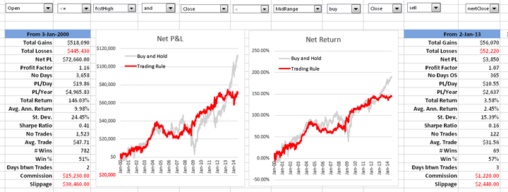
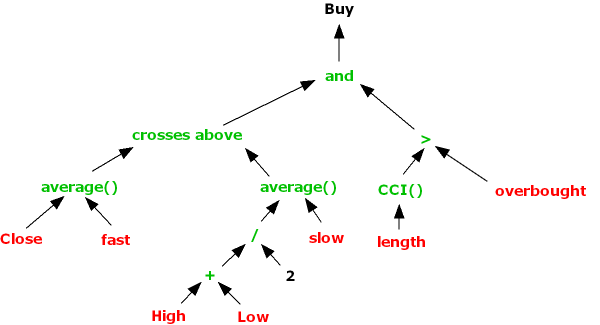
Fig. 1 below shows the summary output from the test for the 3M Company (NYSE:MMM). At the top you can see the best trading rule that the system was able to find for this particular stock. In simple English, the rule tells you to buy today’s close in MMM and sell tomorrow’s close, if the stock opened below the forecast of yesterday’s high price and, in addition, the stock closed below the midrange of the day (the average of today’s high and low prices).
Fig. 1 Summary Analysis for MMM

Source: Yahoo Finance.
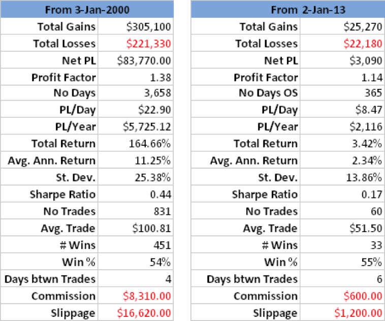
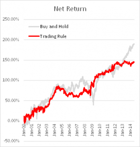
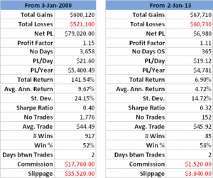
The in-sample results from Jan 2000, summarized in left-hand table in Fig. 2 below, are hardly stellar, but do show evidence of a small, but significant edge, with total net returns of 165%, profit factor of 1.38 and % win rate of 54%. And while the trading rule is, ultimately, outperformed by a simple buy-and-hold strategy, after taking into account transaction costs, for extended periods (e.g. 2009-2012), investors would have been better off had they used the trading rule, because it successfully avoided the worst of the effects of the 2008/09 market crash.
Out-of-sample results, shown in the right-hand table, are less encouraging, but net returns are nonetheless positive and the % win rate actually increases to 55%.
Fig 2. Trade Rule Performance

Source: Yahoo Finance.
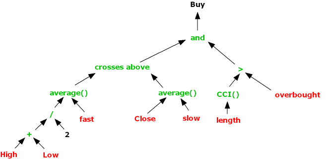
I noted earlier that the first part of our trading rule for MMM involved comparing the opening price to the forecast of yesterday’s high, produced by the vector autoregression model, while the second part of the trading rule references only the midrange and closing prices. How much added value does the VAR model provide? We can test this by eliminating the first part of the rule and considering all days in which the stock closed below the midrange. The results turn out to as shown in Fig. 3.
Fig. 3 Performance of Simplified Trading Rule
Source: Yahoo Finance.
As expected, the in-sample results from our shortened trading rule are certainly inferior to the original rule, in which the VAR model forecasts played a role. But the out-of-sample performance of the simplified rule is actually improved – not only is the net return higher than before, so too is the % win rate, by a couple of percentage points.
A similar pattern emerges for many other stocks: in almost every case, our test algorithm finds that the best trading rule buys the close, based on a comparison of the closing price to the mid-range price. In some cases, the in-sample test results are improved by adding further conditions, such as we saw in the case of MMM. But, as with MMM, we often find that the additional benefit derived from use of the autoregression model forecasts fails to improve trading rule results in the out-of-sample period, and indeed often makes them worse.
Conclusion
In general, we find evidence that a simple trading rule based on a comparison of the closing price to the mid-range price appears to work for many stocks, across long time spans.
In a sense, this simple trading rule is already well known: it is just a variant of the “buy the dips” idea, where, in this case, we define a dip as being when the stock closes below the mid-range of the day, rather than, say, below a moving average level. The economic basis for this finding is also well known: stocks have positive drift. But it is interesting to find yet another confirmation of this well-known idea. And it leaves open the possibility that the trading concept could be further improved by introducing additional rules, trading indicators, and model forecasts to the mix.