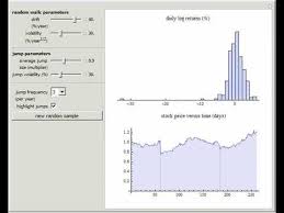
The “implied volatility” corresponding to an option price is the value of the volatility parameter for which the Black-Scholes model gives the same price. A well-known phenomenon in market option prices is the “volatility smile”, in which the implied volatility increases for strike values away from the spot price. The jump diffusion model is a generalization of Black\[Dash]Scholes in which the stock price has randomly occurring jumps in addition to the random walk behavior. One of the interesting properties of this model is that it displays the volatility smile effect. In this Demonstration, we explore the Black-Scholes implied volatility of option prices (equal for both put and call options) in the jump diffusion model. The implied volatility is modeled as a function of the ratio of option strike price to spot price.
The research in this post and the related paper on Range Based EGARCH Option pricing Models is focused on the innovative range-based volatility models introduced in Alizadeh, Brandt, and Diebold (2002) (hereafter ABD). We develop new option pricing models using multi-factor diffusion approximations couched within this theoretical framework and examine their properties in comparison with the traditional Black-Scholes model.
The two-factor version of the model, which I have applied successfully in various option arbitrage strategies, encapsulates the intuively appealing idea of a trending long term mean volatility process, around which oscillates a mean-reverting, transient volatility process. The option pricing model also incorporates asymmetry/leverage effects and well as correlation effects between the asset return and volatility processes, which results in a volatility skew.
The core concept behind Range-Based Exponential GARCH model is Log-Range estimator discussed in an earlier post on volatility metrics, which contains a lengthy exposition of various volatility estimators and their properties. (Incidentally, for those of you who requested a copy of my paper on Estimating Historical Volatility, I have updated the post to include a link to the pdf).
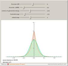
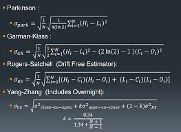
We assume that the log stock price s follows a drift-less Brownian motion ds = sdW. The volatility of daily log returns, denoted h= s/sqrt(252), is assumed constant within each day, at ht from the beginning to the end of day t, but is allowed to change from one day to the next, from ht at the end of day t to ht+1 at the beginning of day t+1. Under these assumptions, ABD show that the log range, defined as:
is to a very good approximation distributed as
where N[m; v] denotes a Gaussian distribution with mean m and variance v. The above equation demonstrates that the log range is a noisy linear proxy of log volatility ln ht. By contrast, according to the results of Alizadeh, Brandt,and Diebold (2002), the log absolute return has a mean of 0.64 + ln ht and a variance of 1.11. However, the distribution of the log absolute return is far from Gaussian. The fact that both the log range and the log absolute return are linear log volatility proxies (with the same loading of one), but that the standard deviation of the log range is about one-quarter of the standard deviation of the log absolute return, makes clear that the range is a much more informative volatility proxy. It also makes sense of the finding of Andersen and Bollerslev (1998) that the daily range has approximately the same informational content as sampling intra-daily returns every four hours.
Except for the model of Chou (2001), GARCH-type volatility models rely on squared or absolute returns (which have the same information content) to capture variation in the conditional volatility ht. Since the range is a more informative volatility proxy, it makes sense to consider range-based GARCH models, in which the range is used in place of squared or absolute returns to capture variation in the conditional volatility. This is particularly true for the EGARCH framework of Nelson (1990), which describes the dynamics of log volatility (of which the log range is a linear proxy).
ABD consider variants of the EGARCH framework introduced by Nelson (1990). In general, an EGARCH(1,1) model performs comparably to the GARCH(1,1) model of Bollerslev (1987). However, for stock indices the in-sample evidence reported by Hentschel (1995) and the forecasting performance presented by Pagan and Schwert (1990) show a slight superiority of the EGARCH specification. One reason for this superiority is that EGARCH models can accommodate asymmetric volatility (often called the “leverage effect,” which refers to one of the explanations of asymmetric volatility), where increases in volatility are associated more often with large negative returns than with equally large positive returns.
The one-factor range-based model (REGARCH 1) takes the form:
where the returns process Rt is conditionally Gaussian: Rt ~ N[0, ht2]
and the process innovation is defined as the standardized deviation of the log range from its expected value:
Following Engle and Lee (1999), ABD also consider multi-factor volatility models. In particular, for a two-factor range-based EGARCH model (REGARCH2), the conditional volatility dynamics) are as follows:
and
where ln qt can be interpreted as a slowly-moving stochastic mean around which log volatility ln ht makes large but transient deviations (with a process determined by the parameters kh, fh and dh).
The parameters q, kq, fq and dq determine the long-run mean, sensitivity of the long run mean to lagged absolute returns, and the asymmetry of absolute return sensitivity respectively.
The intuition is that when the lagged absolute return is large (small) relative to the lagged level of volatility, volatility is likely to have experienced a positive (negative) innovation. Unfortunately, as we explained above, the absolute return is a rather noisy proxy of volatility, suggesting that a substantial part of the volatility variation in GARCH-type models is driven by proxy noise as opposed to true information about volatility. In other words, the noise in the volatility proxy introduces noise in the implied volatility process. In a volatility forecasting context, this noise in the implied volatility process deteriorates the quality of the forecasts through less precise parameter estimates and, more importantly, through less precise estimates of the current level of volatility to which the forecasts are anchored.
As regards the question of forecasting accuracy discussed in the paper on Forecasting Volatility in the S&P 500 Index, there are two possible misunderstandings here that need to be cleared up. These arise from remarks by one commentator as follows:
“An above 50% vol direction forecast looks good,.. but “direction” is biased when working with highly skewed distributions! ..so it would be nice if you could benchmark it against a simple naive predictors to get a feel for significance, -or- benchmark it with a trading strategy and see how the risk/return performs.”
(i) The first point is simple, but needs saying: the phrase “skewed distributions” in the context of volatility modeling could easily be misconstrued as referring to the volatility skew. This, of course, is used to describe to the higher implied vols seen in the Black-Scholes prices of OTM options. But in the Black-Scholes framework volatility is constant, not stochastic, and the “skew” referred to arises in the distribution of the asset return process, which has heavier tails than the Normal distribution (excess Kurtosis and/or skewness). I realize that this is probably not what the commentator meant, but nonetheless it’s worth heading that possible misunderstanding off at the pass, before we go on.
(ii) I assume that the commentator was referring to the skewness in the volatility process, which is characterized by the LogNormal distribution. But the forecasting tests referenced in the paper are tests of the ability of the model to predict the direction of volatility, i.e. the sign of the change in the level of volatility from the current period to the next period. Thus we are looking at, not a LogNormal distribution, but the difference in two LogNormal distributions with equal mean – and this, of course, has an expectation of zero. In other words, the expected level of volatility for the next period is the same as the current period and the expected change in the level of volatility is zero. You can test this very easily for yourself by generating a large number of observations from a LogNormal process, taking the difference and counting the number of positive and negative changes in the level of volatility from one period to the next. You will find, on average, half the time the change of direction is positive and half the time it is negative.
For instance, the following chart shows the distribution of the number of positive changes in the level of a LogNormally distributed random variable with mean and standard deviation of 0.5, for a sample of 1,000 simulations, each of 10,000 observations. The sample mean (5,000.4) is very close to the expected value of 5,000.
Distribution Number of Positive Direction Changes
So, a naive predictor will forecast volatility to remain unchanged for the next period and by random chance approximately half the time volatility will turn out to be higher and half the time it will turn out to be lower than in the current period. Hence the default probability estimate for a positive change of direction is 50% and you would expect to be right approximately half of the time. In other words, the direction prediction accuracy of the naive predictor is 50%. This, then, is one of the key benchmarks you use to assess the ability of the model to predict market direction. That is what test statistics like Theil’s-U does – measures the performance relative to the naive predictor. The other benchmark we use is the change of direction predicted by the implied volatility of ATM options.
In this context, the model’s 61% or higher direction prediction accuracy is very significant (at the 4% level in fact) and this is reflected in the Theil’s-U statistic of 0.82 (lower is better). By contrast, Theil’s-U for the Implied Volatility forecast is 1.46, meaning that IV is a much worse predictor of 1-period-ahead changes in volatility than the naive predictor.
On its face, it is because of this exceptional direction prediction accuracy that a simple strategy is able to generate what appear to be abnormal returns using the change of direction forecasts generated by the model, as described in the paper. In fact, the situation is more complicated than that, once you introduce the concept of a market price of volatility risk.
This post covers quite a wide range of concepts in volatility modeling relating to long memory and regime shifts and is based on an article that was published in Wilmott magazine and republished in The Best of Wilmott Vol 1 in 2005. A copy of the article can be downloaded here.
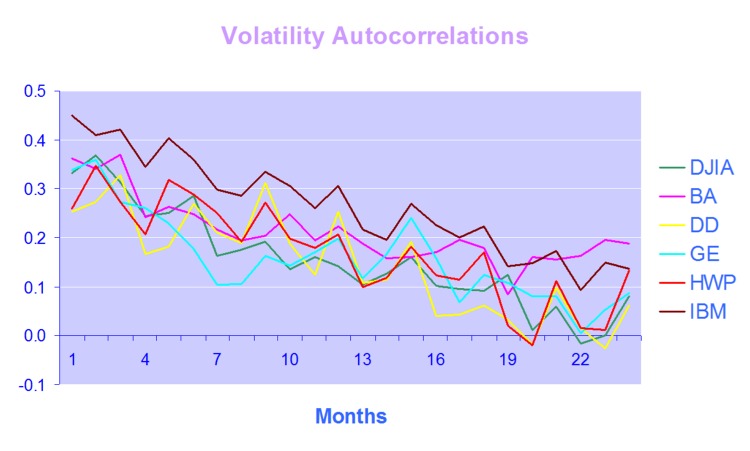
One of the defining characteristics of volatility processes in general (not just financial assets) is the tendency for the serial autocorrelations to decline very slowly. This effect is illustrated quite clearly in the chart below, which maps the autocorrelations in the volatility processes of several financial assets.
Thus we can say that events in the volatility process for IBM, for instance, continue to exert influence on the process almost two years later.
This feature in one that is typical of a black noise process – not some kind of rap music variant, but rather:
“a process with a 1/fβ spectrum, where β > 2 (Manfred Schroeder, “Fractals, chaos, power laws“). Used in modeling various environmental processes. Is said to be a characteristic of “natural and unnatural catastrophes like floods, droughts, bear markets, and various outrageous outages, such as those of electrical power.” Further, “because of their black spectra, such disasters often come in clusters.”” [Wikipedia].
Because of these autocorrelations, black noise processes tend to reinforce or trend, and hence (to some degree) may be forecastable. This contrasts with a white noise process, such as an asset return process, which has a uniform power spectrum, insignificant serial autocorrelations and no discernable trending behavior:
White Noise Power Spectrum
An econometrician might describe this situation by saying that a black noise process is fractionally integrated order d, where d = H/2, H being the Hurst Exponent. A way to appreciate the difference in the behavior of a black noise process vs. a white process is by comparing two fractionally integrated random walks generated using the same set of quasi random numbers by Feder’s (1988) algorithm (see p 32 of the presentation on Modeling Asset Volatility).
Fractal Random Walk – White NoiseFractal Random Walk – Black Noise Process
As you can see. both random walks follow a similar pattern, but the black noise random walk is much smoother, and the downward trend is more clearly discernible. You can play around with the Feder algorithm, which is coded in the accompanying Excel Workbook on Volatility and Nonlinear Dynamics . Changing the Hurst Exponent parameter H in the worksheet will rerun the algorithm and illustrate a fractal random walk for a black noise (H > 0.5), white noise (H=0.5) and mean-reverting, pink noise (H<0.5) process.
One way of modeling the kind of behavior demonstrated by volatility process is by using long memory models such as ARFIMA and FIGARCH (see pp 47-62 of the Modeling Asset Volatility presentation for a discussion and comparison of various long memory models). The article reviews research into long memory behavior and various techniques for estimating long memory models and the coefficient of fractional integration d for a process.
But long memory is not the only possible cause of long term serial correlation. The same effect can result from structural breaks in the process, which can produce spurious autocorrelations. The article goes on to review some of the statistical procedures that have been developed to detect regime shifts, due to Bai (1997), Bai and Perron (1998) and the Iterative Cumulative Sums of Squares methodology due to Aggarwal, Inclan and Leal (1999). The article illustrates how the ICSS technique accurately identifies two changes of regimes in a synthetic GBM process.
In general, I have found the ICSS test to be a simple and highly informative means of gaining insight about a process representing an individual asset, or indeed an entire market. For example, ICSS detects regime shifts in the process for IBM around 1984 (the time of the introduction of the IBM PC), the automotive industry in the early 1980’s (Chrysler bailout), the banking sector in the late 1980’s (Latin American debt crisis), Asian sector indices in Q3 1997, the S&P 500 index in April 2000 and just about every market imaginable during the 2008 credit crisis. By splitting a series into pre- and post-regime shift sub-series and examining each segment for long memory effects, one can determine the cause of autocorrelations in the process. In some cases, Asian equity indices being one example, long memory effects disappear from the series, indicating that spurious autocorrelations were induced by a major regime shift during the 1997 Asian crisis. In most cases, however, long memory effects persist.
I am planning a series of posts on the subject of asset volatility and option pricing and thought I would begin with a survey of some of the central ideas. The attached presentation on Modeling Asset Volatility sets out the foundation for a number of key concepts and the basis for the research to follow.
Perhaps the most important feature of volatility is that it is stochastic rather than constant, as envisioned in the Black Scholes framework. The presentation addresses this issue by identifying some of the chief stylized facts about volatility processes and how they can be modelled. Certain characteristics of volatility are well known to most analysts, such as, for instance, its tendency to “cluster” in periods of higher and lower volatility. However, there are many other typical features that are less often rehearsed and these too are examined in the presentation.
Long Memory For example, while it is true that GARCH models do a fine job of modeling the clustering effect they typically fail to capture one of the most important features of volatility processes – long term serial autocorrelation. In the typical GARCH model autocorrelations die away approximately exponentially, and historical events are seen to have little influence on the behaviour of the process very far into the future. In volatility processes that is typically not the case, however: autocorrelations die away very slowly and historical events may continue to affect the process many weeks, months or even years ahead.
Volatility Direction Prediction Accuracy
There are two immediate and very important consequences of this feature. The first is that volatility processes will tend to trend over long periods – a characteristic of Black Noise or Fractionally Integrated processes, compared to the White Noise behavior that typically characterizes asset return processes. Secondly, and again in contrast with asset return processes, volatility processes are inherently predictable, being conditioned to a significant degree on past behavior. The presentation considers the fractional integration frameworks as a basis for modeling and forecasting volatility.
Mean Reversion vs. Momentum A puzzling feature of much of the literature on volatility is that it tends to stress the mean-reverting behavior of volatility processes. This appears to contradict the finding that volatility behaves as a reinforcing process, whose long-term serial autocorrelations create a tendency to trend. This leads to one of the most important findings about asset processes in general, and volatility process in particular: i.e. that the assets processes are simultaneously trending and mean-reverting. One way to understand this is to think of volatility, not as a single process, but as the superposition of two processes: a long term process in the mean, which tends to reinforce and trend, around which there operates a second, transient process that has a tendency to produce short term spikes in volatility that decay very quickly. In other words, a transient, mean reverting processes inter-linked with a momentum process in the mean. The presentation discusses two-factor modeling concepts along these lines, and about which I will have more to say later.
Cointegration
One of the most striking developments in econometrics over the last thirty years, cointegration is now a principal weapon of choice routinely used by quantitative analysts to address research issues ranging from statistical arbitrage to portfolio construction and asset allocation. Back in the late 1990’s I and a handful of other researchers realized that volatility processes exhibited very powerful cointegration tendencies that could be harnessed to create long-short volatility strategies, mirroring the approach much beloved by equity hedge fund managers. In fact, this modeling technique provided the basis for the Caissa Capital volatility fund, which I founded in 2002. The presentation examines characteristics of multivariate volatility processes and some of the ideas that have been proposed to model them, such as FIGARCH (fractionally-integrated GARCH).
Dispersion Dynamics Finally, one topic that is not considered in the presentation, but on which I have spent much research effort in recent years, is the behavior of cross-sectional volatility processes, which I like to term dispersion. It turns out that, like its univariate cousin, dispersion displays certain characteristics that in principle make it highly forecastable. Given an appropriate model of dispersion dynamics, the question then becomes how to monetize efficiently the insight that such a model offers. Again, I will have much more to say on this subject, in future.
There has been a good deal of interest in the market timing ideas discussed in my earlier blog post Using Volatility to Predict Market Direction, which discusses the research of Diebold and Christoffersen into the sign predictability induced by volatility dynamics. The ideas are thoroughly explored in a QuantNotes article from 2006, which you can download here.
There is a follow-up article from 2006 in which Christoffersen, Diebold, Mariano and Tay develop the ideas further to consider the impact of higher moments of the asset return distribution on sign predictability and the potential for market timing in international markets (download here).
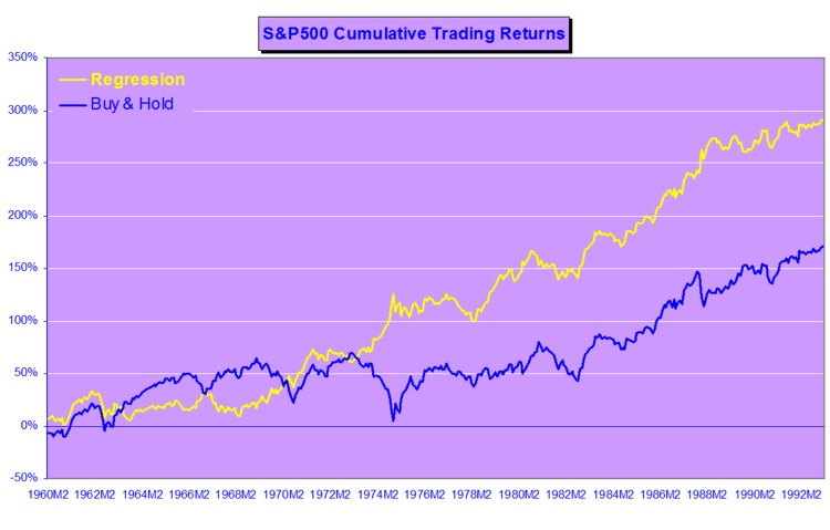
Trading Strategy To illustrate some of the possibilities of this approach, we constructed a simple market timing strategy in which a position was taken in the S&P 500 index or in 90-Day T-Bills, depending on an ex-ante forecast of positive returns from the logit regression model (and using an expanding window to estimate the drift coefficient). We assume that the position is held for 30 days and rebalanced at the end of each period. In this test we make no allowance for market impact, or transaction costs.
Results
Annual returns for the strategy and for the benchmark S&P 500 Index are shown in the figure below. The strategy performs exceptionally well in 1987, 1989 and 1995, when the ratio between expected returns and volatility remains close to optimum levels and the direction of the S&P 500 Index is highly predictable, Of equal interest is that the strategy largely avoids the market downturn of 2000-2002 altogether, a period in which sign probabilities were exceptionally low.
In terms of overall performance, the model enters the market in 113 out of a total of 241 months (47%) and is profitable in 78 of them (69%). The average gain is 7.5% vs. an average loss of –4.11% (ratio 1.83). The compound annual return is 22.63%, with an annual volatility of 17.68%, alpha of 14.9% and Sharpe ratio of 1.10.
The under-performance of the strategy in 2003 is explained by the fact that direction-of-change probabilities were rising from a very low base in Q4 2002 and do not reach trigger levels until the end of the year. Even though the strategy out-performed the Index by a substantial margin of 6% , the performance in 2005 is of concern as market volatility was very low and probabilities overall were on a par with those seen in 1995. Further tests are required to determine whether the failure of the strategy to produce an exceptional performance on par with 1995 was the result of normal statistical variation or due to changes in the underlying structure of the process requiring model recalibration.
Future Research & Development The obvious next step is to develop the approach described above to formulate trading strategies based on sign forecasting in a universe of several assets, possibly trading binary options. The approach also has potential for asset allocation, portfolio theory and risk management applications.
Several people have asked me for copies of this research article, which develops a new theoretical framework, the ARFIMA-GARCH model as a basis for forecasting volatility in the S&P 500 Index. I am in the process of updating the research, but in the meantime a copy of the original paper is available here
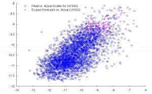
In this analysis we are concerned with the issue of whether market forecasts of volatility, as expressed in the Black-Scholes implied volatilities of at-the-money European options on the S&P500 Index, are superior to those produced by a new forecasting model in the GARCH framework which incorporates long-memory effects. The ARFIMA-GARCH model, which uses high frequency data comprising 5-minute returns, makes volatility the subject process of interest, to which innovations are introduced via a volatility-of-volatility (kurtosis) process. Despite performing robustly in- and out-of-sample, an encompassing regression indicates that the model is unable to add to the information already contained in market forecasts. However, unlike model forecasts, implied volatility forecasts show evidence of a consistent and substantial bias. Furthermore, the model is able to correctly predict the direction of volatility approximately 62% of the time whereas market forecasts have very poor direction prediction ability. This suggests that either option markets may be inefficient, or that the option pricing model is mis-specified. To examine this hypothesis, an empirical test is carried out in which at-the-money straddles are bought or sold (and delta-hedged) depending on whether the model forecasts exceed or fall below implied volatility forecasts. This simple strategy generates an annual compound return of 18.64% over a four year out-of-sample period, during which the annual return on the S&P index itself was -7.24%. Our findings suggest that, over the period of analysis, investors required an additional risk premium of 88 basis points of incremental return for each unit of volatility risk.
We can decompose the returns process Rt as follows:
While the left hand side of the equation is essentially unforecastable, both of the right-hand-side components of returns display persistent dynamics and hence are forecastable.Both the signs of returns and magnitude of returns are conditional mean dependent and hence forecastable, but their product is conditional mean independent and hence unforecastable.This is an example of a nonlinear “common feature” in the sense of Engle and Kozicki (1993).
Although asset returns are essentially unforecastable, the same is not true for asset return signs (i.e. the direction-of-change). As long as expected returns are nonzero, one should expect sign dependence, given the overwhelming evidence of volatility dependence. Even in assets where expected returns are zero, sign dependence may be induced by skewness in the asset returns process. Hence market timing ability is a very real possibility, depending on the relationship between the mean of the asset returns process and its higher moments. The highly nonlinear nature of the relationship means that conditional sign dependence is not likely to be found by traditional measures such as signs autocorrelations, runs tests or traditional market timing tests. Sign dependence is likely to be strongest at intermediate horizons of 1-3 months, and unlikely to be important at very low or high frequencies.Empirical tests demonstrate that sign dependence is very much present in actual US equity returns, with probabilities of positive returns rising to 65% or higher at various points over the last 20 years. A simple logit regression model captures the essentials of the relationship very successfully.
Now consider the implications of dependence and hence forecastability in the sign of asset returns, or, equivalently, the direction-of-change. It may be possible to develop profitable trading strategies if one can successfully time the market, regardless of whether or not one is able to forecast the returns themselves.
There is substantial evidence that sign forecasting can often be done successfully. Relevant research on this topic includes Breen, Glosten and Jaganathan (1989), Leitch and Tanner (1991), Wagner, Shellans and Paul (1992), Pesaran and Timmerman (1995), Kuan and Liu (1995), Larsen and Wozniak (10050, Womack (1996), Gencay (1998), Leung Daouk and Chen (1999), Elliott and Ito (1999) White (2000), Pesaran and Timmerman (2000), and Cheung, Chinn and Pascual (2003).
There is also a huge body of empirical research pointing to the conditional dependence and forecastability of asset volatility. Bollerslev, Chou and Kramer (1992) review evidence in the GARCH framework, Ghysels, Harvey and Renault (1996) survey results from stochastic volatility modeling, while Andersen, Bollerslev and Diebold (2003) survey results from realized volatility modeling.
Sign Dynamics Driven By Volatility Dynamics
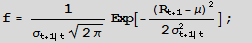
Let the returns process Rt be Normally distributed with mean m and conditional volatility st.
The probability of a positive return Pr[Rt+1>0] is given by the Normal CDF F=1-Prob[0,f]
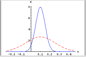
For a given mean return, m, the probability of a positive return is a function of conditional volatility st. As the conditional volatility increases, the probability of a positive return falls, as illustrated in Figure 1 below with m = 10% and st = 5% and 15%.
In the former case, the probability of a positive return is greater because more of the probability mass lies to the right of the origin. Despite having the same, constant expected return of 10%, the process has a greater chance of generating a positive return in the first case than in the second. Thus volatility dynamics drive sign dynamics.
Figure 1
Email me at jkinlay@investment-analytics.com.com for a copy of the complete article.
For a very long time analysts were content to accept the standard deviation of returns as the norm for estimating volatility, even though theoretical research and empirical evidence dating from as long ago as 1980 suggested that superior estimators existed.
Part of the reason was that the claimed efficiency improvements of the Parkinson, Garman–Klass and other estimators failed to translate into practice when applied to real data. Or, at least, no one could quite be sure whether such estimators really were superior when applied to empirical data since volatility, the second moment of the returns distribution, is inherently unknowable. You can say for sure what the return on a particular stock in a particular month was simply by taking the log of the ratio of the stock price at the month end and beginning. But the same cannot be said of volatility: the standard deviation of daily returns during the month, often naively assumed to represent the asset volatility, is in fact only an estimate of it.
Realized Volatility
All that began to change around 2000 with the advent of high frequency data and the concept of Realized Volatility developed by Andersen and others (see Andersen, T.G., T. Bollerslev, F.X. Diebold and P. Labys (2000), “The Distribution of Exchange Rate Volatility,” Revised version of NBER Working Paper No. 6961). The researchers showed that, in principle, one could arrive at an estimate of volatility arbitrarily close to its true value by summing the squares of asset returns at sufficiently high frequency. From this point onwards, Realized Volatility became the “gold standard” of volatility estimation, leaving other estimators in the dust.
Except that, in practice, there are often reasons why Realized Volatility may not be the way to go: for example, high frequency data may not be available for the series, or only for a portion of it; and bid-ask bounce can have a substantial impact on the robustness of Realized Volatility estimates. So even where high frequency data is available, it may still make sense to compute alternative volatility estimators. Indeed, now that a “gold standard” estimator of true volatility exists, it is possible to get one’s arms around the question of the relative performance of other estimators. That was my intent in my research paper on Estimating Historical Volatility, in which I compare the performance characteristics of the Parkinson, Garman–Klass and other estimators relative to the realized volatility estimator. The comparison was made on a number of synthetic GBM processes in which the simulated series incorporated non-zero drift, jumps, and stochastic volatility. A further evaluation was made using an actual data series, comprising 5 minute returns on the S&P 500 in the period from Jan 1988 to Dec 2003.
The findings were generally supportive of the claimed efficiency improvements for all of the estimators, which were superior to the classical standard deviation of returns on every criterion in almost every case. However, the evident superiority of all of the estimators, including the Realized Volatility estimator, began to decline for processes with non-zero drift, jumps and stochastic volatility. There was even evidence of significant bias in some of the estimates produced for some of the series, notably by the standard deviation of returns estimator.
The Log Volatility Estimator
Finally, analysis of the results from the study of the empirical data series suggested that there were additional effects in the empirical data, not seen in the simulated processes, that caused estimator efficiency to fall well below theoretical levels. One conjecture is that long memory effects, a hallmark of most empirical volatility processes, played a significant role in that finding.
The bottom line is that, overall, the log-range volatility estimator performs robustly and with superior efficiency to the standard deviation of returns estimator, regardless of the precise characteristics of the underlying process.


