As markets continue to make new highs against a backdrop of ever diminishing participation and trading volume, investors have legitimate reasons for being concerned about prospects for the remainder of 2016 and beyond, even without consideration to the myriad of economic and geopolitical risks that now confront the US and global economies. Against that backdrop, remaining fully invested is a test of nerves for those whose instinct is that they may be picking up pennies in front an oncoming steamroller. On the other hand, there is a sense of frustration in cashing out, only to watch markets surge another several hundred points to new highs.
In this article I am going to outline some steps investors can take to match their investment portfolios to suit current market conditions in a way that allows them to remain fully invested, while safeguarding against downside risk. In what follows I will be using our own Strategic Volatility Strategy, which invests in volatility ETFs such as the iPath S&P 500 VIX ST Futures ETN (NYSEArca:VXX) and the VelocityShares Daily Inverse VIX ST ETN (NYSEArca:XIV), as an illustrative example, although the principles are no less valid for portfolios comprising other ETFs or equities.

Risk and Volatility
Risk may be defined as the uncertainty of outcome and the most common way of assessing it in the context of investment theory is by means of the standard deviation of returns. One difficulty here is that one may never ascertain the true rate of volatility – the second moment – of a returns process; one can only estimate it. Hence, while one can be certain what the closing price of a stock was at yesterday’s market close, one cannot say what the volatility of the stock was over the preceding week – it cannot be observed the way that a stock price can, only estimated. The most common estimator of asset volatility is, of course, the sample standard deviation. But there are many others that are arguably superior: Log-Range, Parkinson, Garman-Klass to name but a few (a starting point for those interested in such theoretical matters is a research paper entitled Estimating Historical Volatility, Brandt & Kinlay, 2005).
Leaving questions of estimation to one side, one issue with using standard deviation as a measure of risk is that it treats upside and downside risk equally – the “risk” that you might double your money in an investment is regarded no differently than the risk that you might see your investment capital cut in half. This is not, of course, how investors tend to look at things: they typically allocate a far higher cost to downside risk, compared to upside risk.
One way to address the issue is by using a measure of risk known as the semi-deviation. This is estimated in exactly the same way as the standard deviation, except that it is applied only to negative returns. In other words, it seeks to isolate the downside risk alone.
This leads directly to a measure of performance known as the Sortino Ratio. Like the more traditional Sharpe Ratio, the Sortino Ratio is a measure of risk-adjusted performance – the average return produced by an investment per unit of risk. But, whereas the Sharpe Ratio uses the standard deviation as the measure of risk, for the Sortino Ratio we use the semi-deviation. In other words, we are measuring the expected return per unit of downside risk.
There may be a great deal of variation in the upside returns of a strategy that would penalize the risk-adjusted returns, as measured by its Sharpe Ratio. But using the Sortino Ratio, we ignore the upside volatility entirely and focus exclusively on the volatility of negative returns (technically, the returns falling below a given threshold, such as the risk-free rate. Here we are using zero as our benchmark). This is, arguably, closer to the way most investors tend to think about their investment risk and return preferences.
In a scenario where, as an investor, you are particularly concerned about downside risk, it makes sense to focus on downside risk. It follows that, rather than aiming to maximize the Sharpe Ratio of your investment portfolio, you might do better to focus on the Sortino Ratio.
Factor Risk and Correlation Risk
Another type of market risk that is often present in an investment portfolio is correlation risk. This is the risk that your investment portfolio correlates to some other asset or investment index. Such risks are often occluded – hidden from view – only to emerge when least wanted. For example, it might be supposed that a “dollar-neutral” portfolio, i.e. a portfolio comprising equity long and short positions of equal dollar value, might be uncorrelated with the broad equity market indices. It might well be. On the other hand, the portfolio might become correlated with such indices during times of market turbulence; or it might correlate positively with some sector indices and negatively with others; or with market volatility, as measured by the CBOE VIX index, for instance.
Where such dependencies are included by design, they are not a problem; but when they are unintended and latent in the investment portfolio, they often create difficulties. The key here is to test for such dependencies against a variety of risk factors that are likely to be of concern. These might include currency and interest rate risk factors, for example; sector indices; or commodity risk factors such as oil or gold (in a situation where, for example, you are investing a a portfolio of mining stocks). Once an unwanted correlation is identified, the next step is to adjust the portfolio holdings to try to eliminate it. Typically, this can often only be done in the average, meaning that, while there is no correlation bias over the long term, there may be periods of positive, negative, or alternating correlation over shorter time horizons. Either way, it’s important to know.
Using the Strategic Volatility Strategy as an example, we target to maximize the Sortino Ratio, subject also to maintaining very lows levels of correlation to the principal risk factors of concern to us, the S&P 500 and VIX indices. Our aim is to create a portfolio that is broadly impervious to changes in the level of the overall market, or in the level of market volatility.
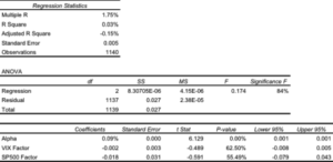
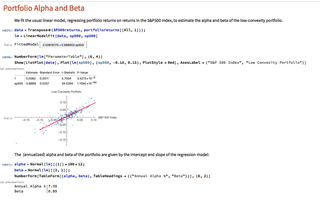
One method of quantifying such dependencies is with linear regression analysis. By way of illustration, in the table below are shown the results of regressing the daily returns from the Strategic Volatility Strategy against the returns in the VIX and S&P 500 indices. Both factor coefficients are statistically indistinguishable from zero, i.e. there is significant no (linear) dependency. However, the constant coefficient, referred to as the strategy alpha, is both positive and statistically significant. In simple terms, the strategy produces a return that is consistently positive, on average, and which is not dependent on changes in the level of the broad market, or its volatility. By contrast, for example, a commonplace volatility strategy that entails capturing the VIX futures roll would show a negative correlation to the VIX index and a positive dependency on the S&P500 index.

Tail Risk
Ever since the publication of Nassim Taleb’s “The Black Swan”, investors have taken a much greater interest in the risk of extreme events. If the bursting of the tech bubble in 2000 was not painful enough, investors surely appear to have learned the lesson thoroughly after the financial crisis of 2008. But even if investors understand the concept, the question remains: what can one do about it?
The place to start is by looking at the fundamental characteristics of the portfolio returns. Here we are not such much concerned with risk, as measured by the second moment, the standard deviation. Instead, we now want to consider the third and forth moments of the distribution, the skewness and kurtosis.
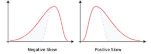
Comparing the two distributions below, we can see that the distribution on the left, with negative skew, has nonzero probability associated with events in the extreme left of the distribution, which in this context, we would associate with negative returns. The distribution on the right, with positive skew, is likewise “heavy-tailed”; but in this case the tail “risk” is associated with large, positive returns. That’s the kind of risk most investors can live with.

Source: Wikipedia
A more direct measure of tail risk is kurtosis, literally, “heavy tailed-ness”, indicating a propensity for extreme events to occur. Again, the shape of the distribution matters: a heavy tail in the right hand portion of the distribution is fine; a heavy tail on the left (indicating the likelihood of large, negative returns) is a no-no.
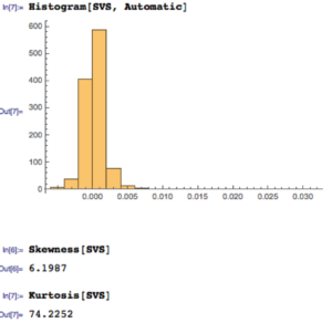
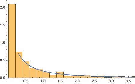
Let’s take a look at the distribution of returns for the Strategic Volatility Strategy. As you can see, the distribution is very positively skewed, with a very heavy right hand tail. In other words, the strategy has a tendency to produce extremely positive returns. That’s the kind of tail risk investors prefer.

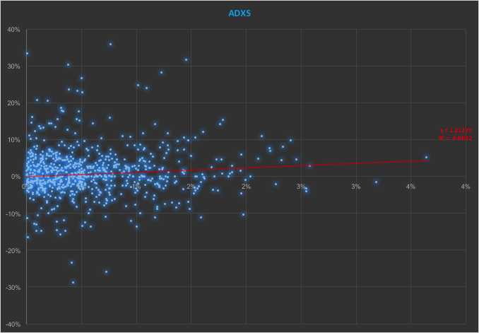
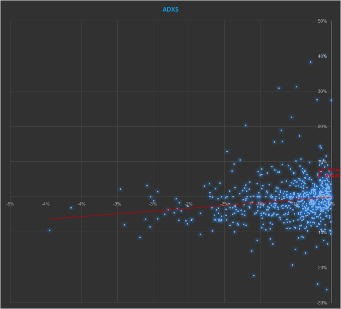
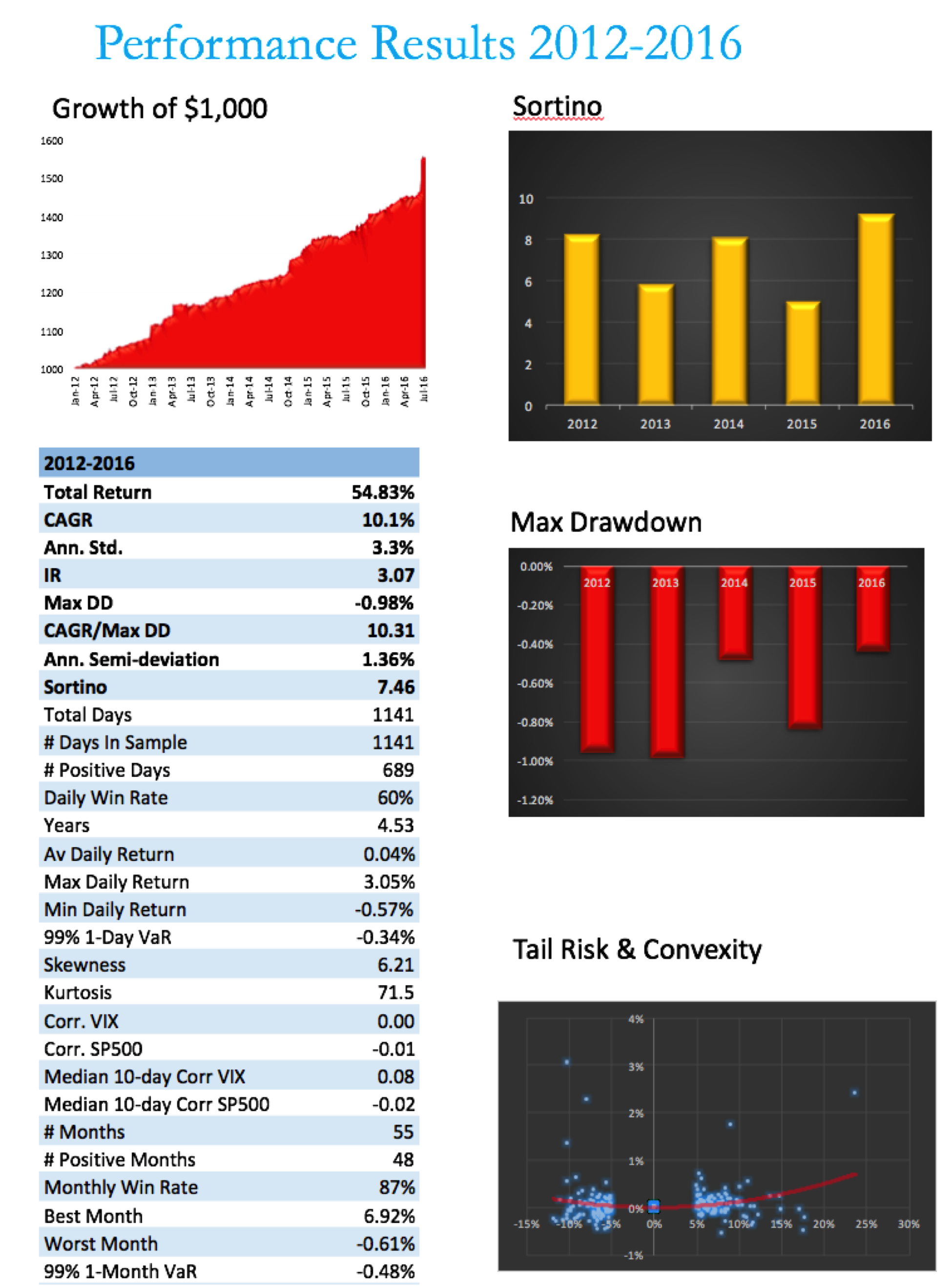
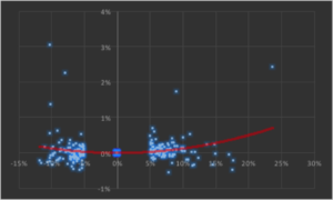
Another way to evaluate tail risk is to examine directly the performance of the strategy during extreme market conditions, when the market makes a major move up or down. Since we are using a volatility strategy as an example, let’s take a look at how it performs on days when the VIX index moves up or down by more than 5%. As you can see from the chart below, by and large the strategy returns on such days tend to be positive and, furthermore, occasionally the strategy produces exceptionally high returns.

The property of producing higher returns to the upside and lower losses to the downside (or, in this case, a tendency to produce positive returns in major market moves in either direction) is known as positive convexity.
Positive convexity, more typically found in fixed income portfolios, is a highly desirable feature, of course. How can it be achieved? Those familiar with options will recognize the convexity feature as being similar to the concept of option Gamma and indeed, one way to produce such a payoff is buy adding options to the investment mix: put options to give positive convexity to the downside, call options to provide positive convexity to the upside (or using a combination of both, i.e. a straddle).
In this case we achieve positive convexity, not by incorporating options, but through a judicious choice of leveraged ETFs, both equity and volatility, for example, the ProShares UltraPro S&P500 ETF (NYSEArca:UPRO) and the ProShares Ultra VIX Short-Term Futures ETN (NYSEArca:UVXY).
Putting It All Together
While we have talked through the various concepts in creating a risk-protected portfolio one-at-a-time, in practice we use nonlinear optimization techniques to construct a portfolio that incorporates all of the desired characteristics simultaneously. This can be a lengthy and tedious procedure, involving lots of trial and error. And it cannot be emphasized enough how important the choice of the investment universe is from the outset. In this case, for instance, it would likely be pointless to target an overall positively convex portfolio without including one or more leveraged ETFs in the investment mix.
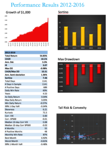
Let’s see how it turned out in the case of the Strategic Volatility Strategy.

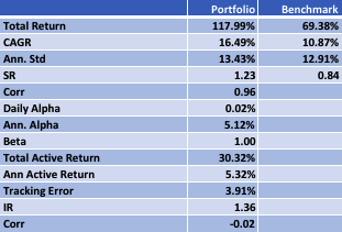
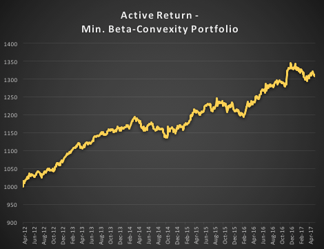
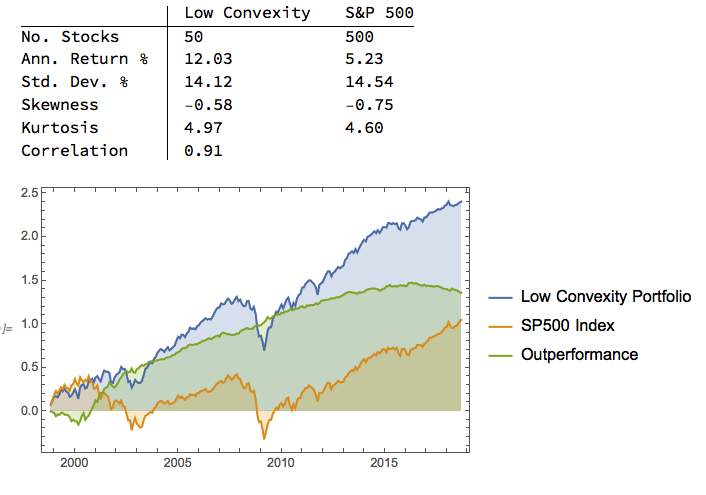
Note that, while the portfolio Information Ratio is moderate (just above 3), the Sortino Ratio is consistently very high, averaging in excess of 7. In large part that is due to the exceptionally low downside risk, which at 1.36% is less than half the standard deviation (which is itself quite low at 3.3%). It is no surprise that the maximum drawdown over the period from 2012 amounts to less than 1%.
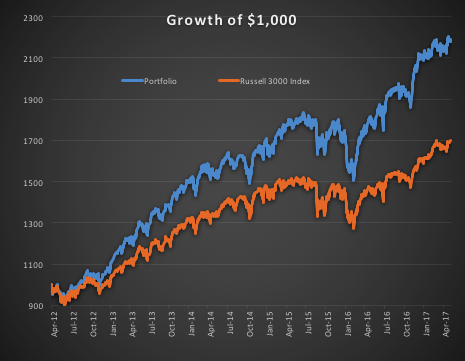
A critic might argue that a CAGR of only 10% is rather modest, especially since market conditions have generally been so benign. I would answer that criticism in two ways. Firstly, this is an investment that has the risk characteristics of a low-duration government bond; and yet it produces a yield many times that of a typical bond in the current low interest rate environment.
Secondly, I would point out that these results are based on use of standard 2:1 Reg-T leverage. In practice it is entirely feasible to increase the leverage up to 4:1, which would produce a CAGR of around 20%. Investors can choose where on the spectrum of risk-return they wish to locate the portfolio and the strategy leverage can be adjusted accordingly.
Conclusion
The current investment environment, characterized by low yields and growing downside risk, poses difficult challenges for investors. A way to address these concerns is to focus on metrics of downside risk in the construction of the investment portfolio, aiming for high Sortino Ratios, low correlation with market risk factors, and positive skewness and convexity in the portfolio returns process.
Such desirable characteristics can be achieved with modern portfolio construction techniques providing the investment universe is chosen carefully and need not include anything more exotic than a collection of commonplace ETF products.


