NOTE: if you are unable to see the Mathematica models below, you can download the free Wolfram CDF player and you may also need this plug-in.
You can also download the complete Mathematica CDF file here.
In this post I want to explore aspects of scalping, a type of strategy widely utilized by high frequency trading firms.
I will define a scalping strategy as one in which we seek to take small profits by posting limit orders on alternate side of the book. Scalping, as I define it, is a strategy rather like market making, except that we “lean” on one side of the book. So, at any given time, we may have a long bias and so look to enter with a limit buy order. If this is filled, we will then look to exit with a subsequent limit sell order, taking a profit of a few ticks. Conversely, we may enter with a limit sell order and look to exit with a limit buy order.
The strategy relies on two critical factors:
(i) the alpha signal which tells us from moment to moment whether we should prefer to be long or short
(ii) the execution strategy, or “trade expression”
In this article I want to focus on the latter, making the assumption that we have some kind of alpha generation model already in place (more about this in later posts).
There are several means that a trader can use to enter a position. The simplest approach, the one we will be considering here, is simply to place a single limit order at or just outside the inside bid/ask prices – so in other words we will be looking to buy on the bid and sell on the ask (and hoping to earn the bid-ask spread, at least).

One of the problems with this approach is that it is highly latency sensitive. Limit orders join the limit order book at the back of the queue and slowly works their way towards the front, as earlier orders get filled. Buy the time the market gets around to your limit buy order, there may be no more sellers at that price. In that case the market trades away, a higher bid comes in and supersedes your order, and you don’t get filled. Conversely, yours may be one of the last orders to get filled, after which the market trades down to a lower bid and your position is immediately under water.
This simplistic model explains why latency is such a concern – you want to get as near to the front of the queue as you can, as quickly as possible. You do this by minimizing the time it takes to issue and order and get it into the limit order book. That entails both hardware (co-located servers, fiber-optic connections) and software optimization and typically also involves the use of Immediate or Cancel (IOC) orders. The use of IOC orders by HFT firms to gain order priority is highly controversial and is seen as gaming the system by traditional investors, who may end up paying higher prices as a result.
Another approach is to layer limit orders at price points up and down the order book, establishing priority long before the market trades there. Order layering is a highly complex execution strategy that brings addition complications.
Let’s confine ourselves to considering the single limit order, the type of order available to any trader using a standard retail platform.
As I have explained, we are assuming here that, at any point in time, you know whether you prefer to be long or short, and therefore whether you want to place a bid or an offer. The issue is, at what price do you place your order, and what do you do about limiting your risk? In other words, we are discussing profit targets and stop losses, which, of course, are all about risk and return.
Risk and Return in Scalping
Lets start by considering risk. The biggest risk to a scalper is that, once filled, the market goes against his position until he is obliged to trigger his stop loss. If he sets his stop loss too tight, he may be forced to exit positions that are initially unprofitable, but which would have recovered and shown a profit if he had not exited. Conversely, if he sets the stop loss too loose, the risk reward ratio is very low – a single loss-making trade could eradicate the profit from a large number of smaller, profitable trades.
Now lets think about reward. If the trader is too ambitious in setting his profit target he may never get to realize the gains his position is showing – the market could reverse, leaving him with a loss on a position that was, initially, profitable. Conversely, if he sets the target too tight, the trader may give up too much potential in a winning trade to overcome the effects of the occasional, large loss.
It’s clear that these are critical concerns for a scalper: indeed the trade exit rules are just as important, or even more important, than the entry rules. So how should he proceed?
Theoretical Framework for Scalping
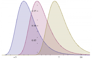
Let’s make the rather heroic assumption that market returns are Normally distributed (in fact, we know from empirical research that they are not – but this is a starting point, at least). And let’s assume for the moment that our trader has been filled on a limit buy order and is looking to decide where to place his profit target and stop loss limit orders. Given a current price of the underlying security of X, the scalper is seeking to determine the profit target of p ticks and the stop loss level of q ticks that will determine the prices at which he should post his limit orders to exit the trade. We can translate these into returns, as follows:
to the upside: Ru = Ln[X+p] – Ln[X]
and to the downside: Rd = Ln[X-q] – Ln[X]
This situation is illustrated in the chart below.
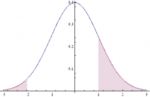
The profitable area is the shaded region on the RHS of the distribution. If the market trades at this price or higher, we will make money: p ticks, less trading fees and commissions, to be precise. Conversely we lose q ticks (plus commissions) if the market trades in the region shaded on the LHS of the distribution.
Under our assumptions, the probability of ending up in the RHS shaded region is:
probWin = 1 – NormalCDF(Ru, mu, sigma),
where mu and sigma are the mean and standard deviation of the distribution.
The probability of losing money, i.e. the shaded area in the LHS of the distribution, is given by:
probLoss = NormalCDF(Rd, mu, sigma),
where NormalCDF is the cumulative distribution function of the Gaussian distribution.
The expected profit from the trade is therefore:
Expected profit = p * probWin – q * probLoss
And the expected win rate, the proportion of profitable trades, is given by:
WinRate = probWin / (probWin + probLoss)
If we set a stretch profit target, then p will be large, and probWin, the shaded region on the RHS of the distribution, will be small, so our winRate will be low. Under this scenario we would have a low probability of a large gain. Conversely, if we set p to, say, 1 tick, and our stop loss q to, say, 20 ticks, the shaded region on the RHS will represent close to half of the probability density, while the shaded LHS will encompass only around 5%. Our win rate in that case would be of the order of 91%:
WinRate = 50% / (50% + 5%) = 91%
Under this scenario, we make frequent, small profits and suffer the occasional large loss.
So the critical question is: how do we pick p and q, our profit target and stop loss? Does it matter? What should the decision depend on?
Modeling Scalping Strategies
We can begin to address these questions by noticing, as we have already seen, that there is a trade-off between the size of profit we are hoping to make, and the size of loss we are willing to tolerate, and the probability of that gain or loss arising. Those probabilities in turn depend on the underlying probability distribution, assumed here to be Gaussian.
Now, the Normal or Gaussian distribution which determines the probabilities of winning or losing at different price levels has two parameters – the mean, mu, or drift of the returns process and sigma, its volatility.
Over short time intervals the effect of volatility outweigh any impact from drift by orders of magnitude. The reason for this is simple: volatility scales with the square root of time, while the drift scales linearly. Over small time intervals, the drift becomes un-noticeably small, compared to the process volatility. Hence we can assume that mu, the process mean is zero, without concern, and focus exclusively on sigma, the volatility.
What other factors do we need to consider? Well there is a minimum price move, which might be 1 tick, and the dollar value of that tick, from which we can derive our upside and downside returns, Ru and Rd. And, finally, we need to factor in commissions and exchange fees into our net trade P&L.
Here’s a simple formulation of the model, in which I am using the E-mini futures contract as an exemplar.
WinRate[currentPrice_,annualVolatility_,BarSizeMins_, nTicksPT_, nTicksSL_,minMove_, tickValue_, costContract_]:=Module[{ nMinsPerDay, periodVolatility, tgtReturn, slReturn,tgtDollar, slDollar, probWin, probLoss, winRate, expWinDollar, expLossDollar, expProfit},
nMinsPerDay = 250*6.5*60;
periodVolatility = annualVolatility / Sqrt[nMinsPerDay/BarSizeMins];
tgtReturn=nTicksPT*minMove/currentPrice;tgtDollar = nTicksPT * tickValue;
slReturn = nTicksSL*minMove/currentPrice;
slDollar=nTicksSL*tickValue;
probWin=1-CDF[NormalDistribution[0, periodVolatility],tgtReturn];
probLoss=CDF[NormalDistribution[0, periodVolatility],slReturn];
winRate=probWin/(probWin+probLoss);
expWinDollar=tgtDollar*probWin;
expLossDollar=slDollar*probLoss;
expProfit=expWinDollar+expLossDollar-costContract;
{expProfit, winRate}]
For the ES contract we have a min price move of 0.25 and the tick value is $12.50. Notice that we scale annual volatility to the size of the period we are trading (15 minute bars, in the following example).
Scenario Analysis
Let’s take a look at how the expected profit and win rate vary with the profit target and stop loss limits we set. In the following interactive graphics, we can assess the impact of different levels of volatility on the outcome.
Expected Profit by Bar Size and Volatility
Expected Win Rate by Volatility
Notice to begin with that the win rate (and expected profit) are very far from being Normally distributed – not least because they change radically with volatility, which is itself time-varying.
For very low levels of volatility, around 5%, we appear to do best in terms of maximizing our expected P&L by setting a tight profit target of a couple of ticks, and a stop loss of around 10 ticks. Our win rate is very high at these levels – around 90% or more. In other words, at low levels of volatility, our aim should be to try to make a large number of small gains.
But as volatility increases to around 15%, it becomes evident that we need to increase our profit target, to around 10 or 11 ticks. The distribution of the expected P&L suggests we have a couple of different strategy options: either we can set a larger stop loss, of around 30 ticks, or we can head in the other direction, and set a very low stop loss of perhaps just 1-2 ticks. This later strategy is, in fact, the mirror image of our low-volatility strategy: at higher levels of volatility, we are aiming to make occasional, large gains and we are willing to pay the price of sustaining repeated small stop-losses. Our win rate, although still well above 50%, naturally declines.
As volatility rises still further, to 20% or 30%, or more, it becomes apparent that we really have no alternative but to aim for occasional large gains, by increasing our profit target and tightening stop loss limits. Our win rate under this strategy scenario will be much lower – around 30% or less.
Non – Gaussian Model
Now let’s address the concern that asset returns are not typically distributed Normally. In particular, the empirical distribution of returns tends to have “fat tails”, i.e. the probability of an extreme event is much higher than in an equivalent Normal distribution.
A widely used model for fat-tailed distributions in the Extreme Value Distribution. This has pdf:
PDF[ExtremeValueDistribution[,],x]

Plot[Evaluate@Table[PDF[ExtremeValueDistribution[,2],x],{,{-3,0,4}}],{x,-8,12},FillingAxis]
Mean[ExtremeValueDistribution[,]]
+EulerGamma
Variance[ExtremeValueDistribution[,]]

In order to set the parameters of the EVD, we need to arrange them so that the mean and variance match those of the equivalent Gaussian distribution with mean = 0 and standard deviation . hence:
The code for a version of the model using the GED is given as follows
WinRateExtreme[currentPrice_,annualVolatility_,BarSizeMins_, nTicksPT_, nTicksSL_,minMove_, tickValue_, costContract_]:=Module[{ nMinsPerDay, periodVolatility, alpha, beta,tgtReturn, slReturn,tgtDollar, slDollar, probWin, probLoss, winRate, expWinDollar, expLossDollar, expProfit},
nMinsPerDay = 250*6.5*60;
periodVolatility = annualVolatility / Sqrt[nMinsPerDay/BarSizeMins];
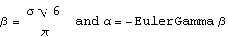
beta = Sqrt[6]*periodVolatility / Pi;
alpha=-EulerGamma*beta;
tgtReturn=nTicksPT*minMove/currentPrice;tgtDollar = nTicksPT * tickValue;
slReturn = nTicksSL*minMove/currentPrice;
slDollar=nTicksSL*tickValue;
probWin=1-CDF[ExtremeValueDistribution[alpha, beta],tgtReturn];
probLoss=CDF[ExtremeValueDistribution[alpha, beta],slReturn];
winRate=probWin/(probWin+probLoss);
expWinDollar=tgtDollar*probWin;
expLossDollar=slDollar*probLoss;
expProfit=expWinDollar+expLossDollar-costContract;
{expProfit, winRate}]
WinRateExtreme[1900,0.05,15,2,30,0.25,12.50,3][[2]]
0.21759
We can now produce the same plots for the EVD version of the model that we plotted for the Gaussian versions :
Expected Profit by Bar Size and Volatility – Extreme Value Distribution
Expected Win Rate by Volatility – Extreme Value Distribution
Next we compare the Gaussian and EVD versions of the model, to gain an understanding of how the differing assumptions impact the expected Win Rate.
Expected Win Rate by Stop Loss and Profit Target
As you can see, for moderate levels of volatility, up to around 18 % annually, the expected Win Rate is actually higher if we assume an Extreme Value distribution of returns, rather than a Normal distribution.If we use a Normal distribution we will actually underestimate the Win Rate, if the actual return distribution is closer to Extreme Value.In other words, the assumption of a Gaussian distribution for returns is actually conservative.
Now, on the other hand, it is also the case that at higher levels of volatility the assumption of Normality will tend to over – estimate the expected Win Rate, if returns actually follow an extreme value distribution. But, as indicated before, for high levels of volatility we need to consider amending the scalping strategy very substantially. Either we need to reverse it, setting larger Profit Targets and tighter Stops, or we need to stop trading altogether, until volatility declines to normal levels.Many scalpers would prefer the second option, as the first alternative doesn’t strike them as being close enough to scalping to justify the name.If you take that approach, i.e.stop trying to scalp in periods when volatility is elevated, then the differences in estimated Win Rate resulting from alternative assumptions of return distribution are irrelevant.
If you only try to scalp when volatility is under, say, 20 % and you use a Gaussian distribution in your scalping model, you will only ever typically under – estimate your actual expected Win Rate.In other words, the assumption of Normality helps, not hurts, your strategy, by being conservative in its estimate of the expected Win Rate.
If, in the alternative, you want to trade the strategy regardless of the level of volatility, then by all means use something like an Extreme Value distribution in your model, as I have done here.That changes the estimates of expected Win Rate that the model produces, but it in no way changes the structure of the model, or invalidates it.It’ s just a different, arguably more realistic set of assumptions pertaining to situations of elevated volatility.
Monte-Carlo Simulation Analysis
Let’ s move on to do some simulation analysis so we can get an understanding of the distribution of the expected Win Rate and Avg Trade PL for our two alternative models. We begin by coding a generator that produces a sample of 1,000 trades and calculates the Avg Trade PL and Win Rate.
Gaussian Model
GenWinRate[currentPrice_,annualVolatility_,BarSizeMins_, nTicksPT_, nTicksSL_,minMove_, tickValue_, costContract_]:=Module[{ nMinsPerDay, periodVolatility, randObs, tgtReturn, slReturn,tgtDollar, slDollar, nWins,nLosses, perTradePL, probWin, probLoss, winRate, expWinDollar, expLossDollar, expProfit},
nMinsPerDay = 250*6.5*60;
periodVolatility = annualVolatility / Sqrt[nMinsPerDay/BarSizeMins];
tgtReturn=nTicksPT*minMove/currentPrice;tgtDollar = nTicksPT * tickValue;
slReturn = nTicksSL*minMove/currentPrice;
slDollar=nTicksSL*tickValue;
randObs=RandomVariate[NormalDistribution[0,periodVolatility],10^3];
nWins=Count[randObs,x_/;x>=tgtReturn];
nLosses=Count[randObs,x_/;xslReturn];
winRate=nWins/(nWins+nLosses)//N;
perTradePL=(nWins*tgtDollar+nLosses*slDollar)/(nWins+nLosses);{perTradePL,winRate}]
GenWinRate[1900,0.1,15,1,-24,0.25,12.50,3]
{7.69231,0.984615}
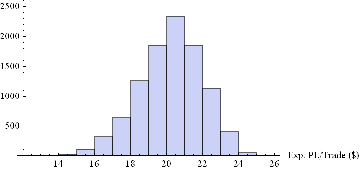
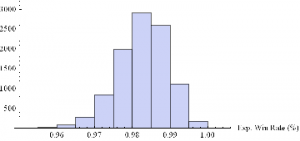
Now we can generate a random sample of 10, 000 simulation runs and plot a histogram of the Win Rates, using, for example, ES on 5-min bars, with a PT of 2 ticks and SL of – 20 ticks, assuming annual volatility of 15 %.
Histogram[Table[GenWinRate[1900,0.15,5,2,-20,0.25,12.50,3][[2]],{i,10000}],10,AxesLabel{“Exp. Win Rate (%)”}]
Histogram[Table[GenWinRate[1900,0.15,5,2,-20,0.25,12.50,3][[1]],{i,10000}],10,AxesLabel{“Exp. PL/Trade ($)”}]

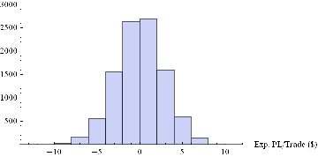
Extreme Value Distribution Model
Next we can do the same for the Extreme Value Distribution version of the model.
GenWinRateExtreme[currentPrice_,annualVolatility_,BarSizeMins_, nTicksPT_, nTicksSL_,minMove_, tickValue_, costContract_]:=Module[{ nMinsPerDay, periodVolatility, randObs, tgtReturn, slReturn,tgtDollar, slDollar, alpha, beta,nWins,nLosses, perTradePL, probWin, probLoss, winRate, expWinDollar, expLossDollar, expProfit},
nMinsPerDay = 250*6.5*60;
periodVolatility = annualVolatility / Sqrt[nMinsPerDay/BarSizeMins];
beta = Sqrt[6]*periodVolatility / Pi;
alpha=-EulerGamma*beta;
tgtReturn=nTicksPT*minMove/currentPrice;tgtDollar = nTicksPT * tickValue;
slReturn = nTicksSL*minMove/currentPrice;
slDollar=nTicksSL*tickValue;
randObs=RandomVariate[ExtremeValueDistribution[alpha, beta],10^3];
nWins=Count[randObs,x_/;x>=tgtReturn];
nLosses=Count[randObs,x_/;xslReturn];
winRate=nWins/(nWins+nLosses)//N;
perTradePL=(nWins*tgtDollar+nLosses*slDollar)/(nWins+nLosses);{perTradePL,winRate}]
Histogram[Table[GenWinRateExtreme[1900,0.15,5,2,-10,0.25,12.50,3][[2]],{i,10000}],10,AxesLabel{“Exp. Win Rate (%)”}]
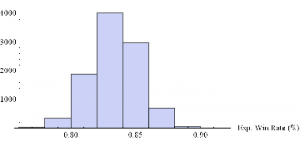
Histogram[Table[GenWinRateExtreme[1900,0.15,5,2,-10,0.25,12.50,3][[1]],{i,10000}],10,AxesLabel{“Exp. PL/Trade ($)”}]

Conclusions
The key conclusions from this analysis are:
- Scalping is essentially a volatility trade
- The setting of optimal profit targets are stop loss limits depend critically on the volatility of the underlying, and needs to be handled dynamically, depending on current levels of market volatility
- At low levels of volatility we should set tight profit targets and wide stop loss limits, looking to make a high percentage of small gains, of perhaps 2-3 ticks.
- As volatility rises, we need to reverse that position, setting more ambitious profit targets and tight stops, aiming for the occasional big win.

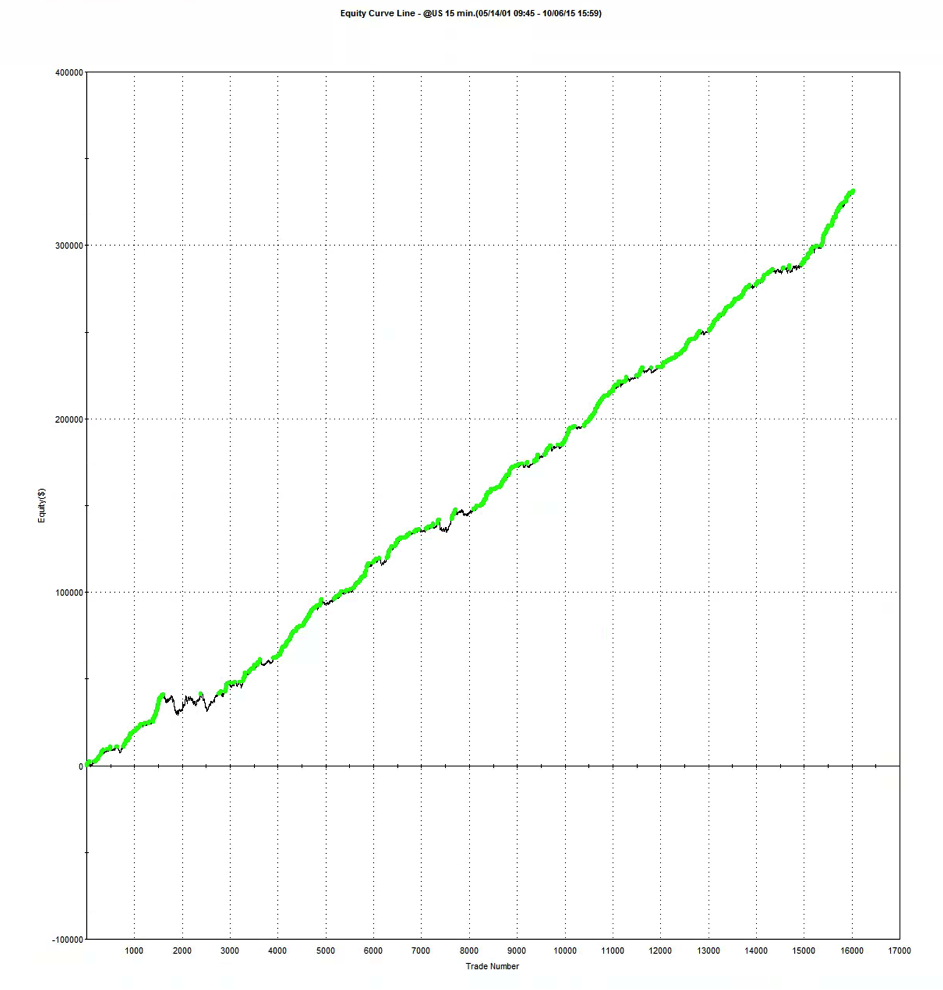
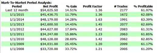
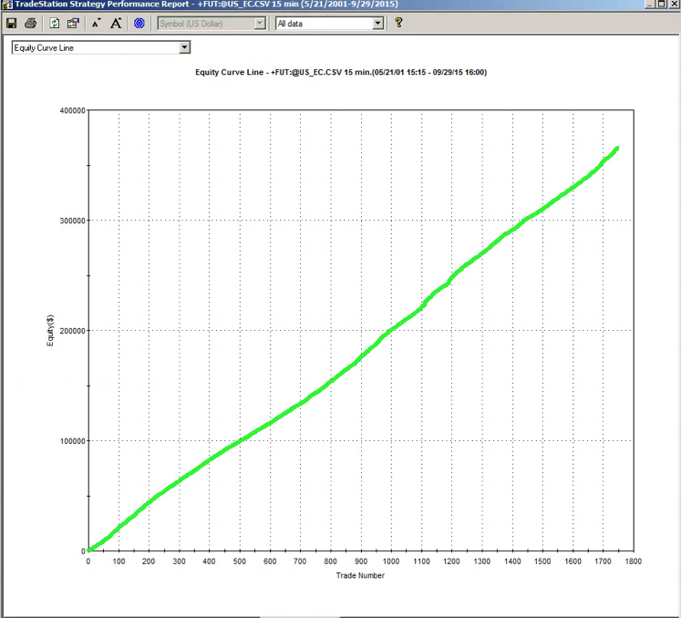
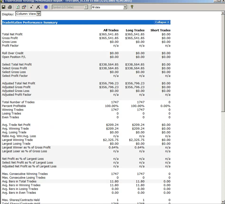
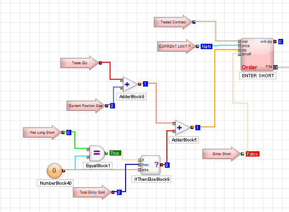
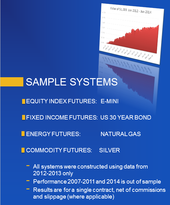
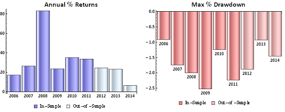
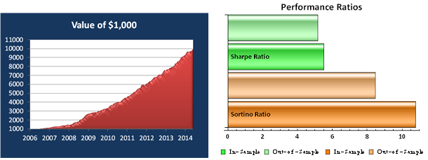
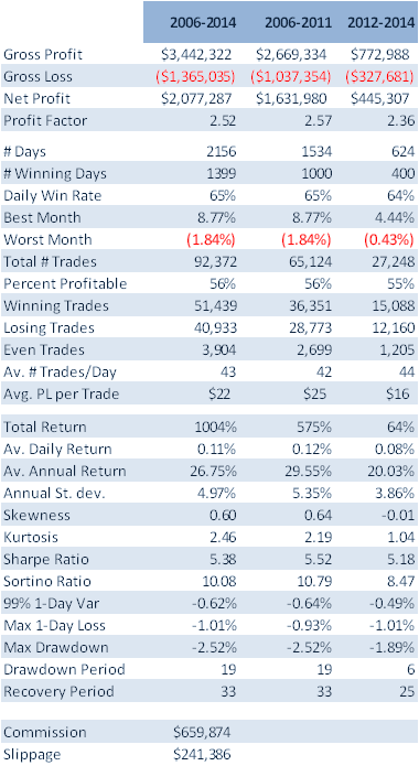
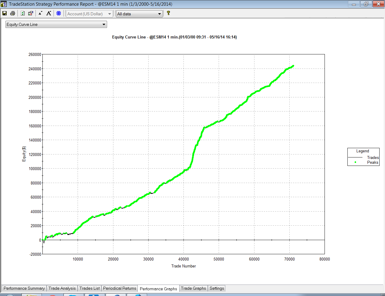
 A meta-strategy is a trading system that trades trading systems. The idea is to develop a strategy that will make sensible decisions about when to trade a specific system, in a way that yields superior performance compared to simply following the underlying trading system. Put another way, the simplest kind of meta-strategy is a long-only strategy that takes positions in some underlying trading system. At times, it will follow the underlying system exactly; at other times it is out of the market and ignore the trading system’s recommendations.