Recently I have been working on the problem of how to construct large portfolios of cointegrated securities. My focus has been on ETFs rather that stocks, although in principle the methodology applies equally well to either, of course.
My preference for ETFs is due primarily to the fact that it is easier to achieve a wide diversification in the portfolio with a more limited number of securities: trading just a handful of ETFs one can easily gain exposure, not only to the US equity market, but also international equity markets, currencies, real estate, metals and commodities. Survivorship bias, shorting restrictions and security-specific risk are also less of an issue with ETFs than with stocks (although these problems are not too difficult to handle).
On the downside, with few exceptions ETFs tend to have much shorter histories than equities or commodities. One also has to pay close attention to the issue of liquidity. That said, I managed to assemble a universe of 85 ETF products with histories from 2006 that have sufficient liquidity collectively to easily absorb an investment of several hundreds of millions of dollars, at minimum.
The Cardinality Problem
The basic methodology for constructing a long/short portfolio using cointegration is covered in an earlier post. But problems arise when trying to extend the universe of underlying securities. There are two challenges that need to be overcome.

The first issue is that, other than the simple regression approach, more advanced techniques such as the Johansen test are unable to handle data sets comprising more than about a dozen securities. The second issue is that the number of possible combinations of cointegrated securities quickly becomes unmanageable as the size of the universe grows. In this case, even taking a subset of just six securities from the ETF universe gives rise to a total of over 437 million possible combinations (85! / (79! * 6!). An exhaustive test of all the possible combinations of a larger portfolio of, say, 20 ETFs, would entail examining around 1.4E+19 possibilities.
Given the scale of the computational problem, how to proceed? One approach to addressing the cardinality issue is sparse canonical correlation analysis, as described in Identifying Small Mean Reverting Portfolios, d’Aspremont (2008). The essence of the idea is something like this. Suppose you find that, in a smaller, computable universe consisting of just two securities, a portfolio comprising, say, SPY and QQQ was found to be cointegrated. Then, when extending consideration to portfolios of three securities, instead of examining every possible combination, you might instead restrict your search to only those portfolios which contain SPY and QQQ. Having fixed the first two selections, you are left with only 83 possible combinations of three securities to consider. This process is repeated as you move from portfolios comprising 3 securities to 4, 5, 6, … etc.
Other approaches to the cardinality problem are possible. In their 2014 paper Sparse, mean reverting portfolio selection using simulated annealing, the Hungarian researchers Norbert Fogarasi and Janos Levendovszky consider a new optimization approach based on simulated annealing. I have developed my own, hybrid approach to portfolio construction that makes use of similar analytical methodologies. Does it work?
A Cointegrated Long/Short ETF Basket
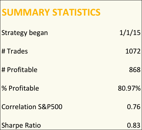
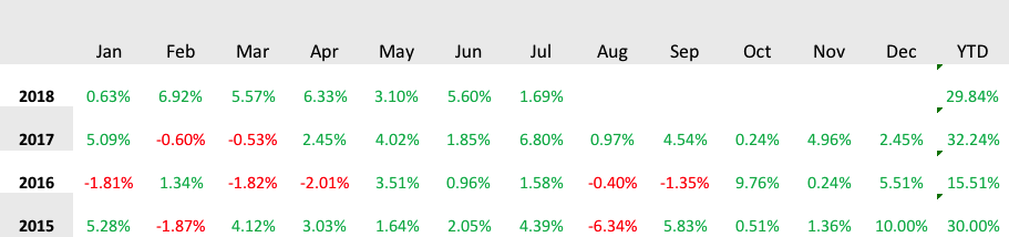
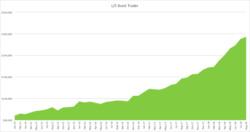
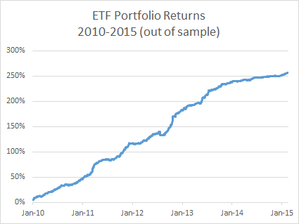
Below are summarized the out-of-sample results for a portfolio comprising 21 cointegrated ETFs over the period from 2010 to 2015. The basket has broad exposure (long and short) to US and international equities, real estate, currencies and interest rates, as well as exposure in banking, oil and gas and other specific sectors.
The portfolio was constructed using daily data from 2006 – 2009, and cointegration vectors were re-computed annually using data up to the end of the prior year. I followed my usual practice of using daily data comprising “closing” prices around 12pm, i.e. in the middle of the trading session, in preference to prices at the 4pm market close. Although liquidity at that time is often lower than at the close, volatility also tends to be muted and one has a period of perhaps as much at two hours to try to achieve the arrival price. I find this to be a more reliable assumption that the usual alternative.
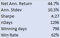
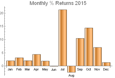
 The risk-adjusted performance of the strategy is consistently outstanding throughout the out-of-sample period from 2010. After a slowdown in 2014, strategy performance in the first quarter of 2015 has again accelerated to the level achieved in earlier years (i.e. with a Sharpe ratio above 4).
Another useful test procedure is to compare the strategy performance with that of a portfolio constructed using standard mean-variance optimization (using the same ETF universe, of course). The test indicates that a portfolio constructed using the traditional Markowitz approach produces a similar annual return, but with 2.5x the annual volatility (i.e. a Sharpe ratio of only 1.6). What is impressive about this result is that the comparison one is making is between the out-of-sample performance of the strategy vs. the in-sample performance of a portfolio constructed using all of the available data.
Having demonstrated the validity of the methodology, at least to my own satisfaction, the next step is to deploy the strategy and test it in a live environment. This is now under way, using execution algos that are designed to minimize the implementation shortfall (i.e to minimize any difference between the theoretical and live performance of the strategy). So far the implementation appears to be working very well.
Once a track record has been built and audited, the really hard work begins: raising investment capital!