Machine Learning Archives - Page 2 of 2 - QUANTITATIVE RESEARCH AND TRADING

February 18, 2020

Futures WealthBuilder – June 2017: +4.4%

The Futures WealthBuilder product is an algorithmic CTA strategy that trades several highly liquid futures contracts using machine learning algorithms. More details about the strategy are given in this blog post.

We offer a version of the strategy on the Collective 2 site (see here for details) that the user can subscribe to for a very modest fee of only $149 per month. The Collective 2 version of the strategy is unlikely to perform as well as the product we offer in our Systematic Strategies Fund, which trades a much wider range of futures products. But the strategy is off to an excellent start, making +4.4% in June and is now up 6.7% since inception in May. In June the strategy made profitable trades in US Bonds, Euro F/X and VIX futures, and the last seven trades in a row have been winners.

You can find full details of the strategy, including a listing of all of the trades, on the Collective 2 site.

Subscribers can sign up for a free, seven day trial and thereafter they can choose to trade the strategy automatically in their own brokerage account, using the Collective 2 api.

January 14, 2020

Futures WealthBuilder

We are launching a new product, the Futures WealthBuilder, a CTA system that trades futures contracts in several highly liquid financial and commodity markets, including SP500 EMinis, Euros, VIX, Gold, US Bonds, 10-year and five-year notes, Corn, Natural Gas and Crude Oil. Each component strategy uses a variety of machine learning algorithms to detect trends, seasonal effects and mean-reversion. We develop several different types of model for each market, and deploy them according to their suitability for current market conditions.

Performance of the strategy (net of fees) since 2013 is detailed in the charts and tables below. Notable features include a Sharpe Ratio of just over 2, an annual rate of return of 190% on an account size of $50,000, and a maximum drawdown of around 8% over the last three years. It is worth mentioning, too, that the strategy produces approximately equal rates of return on both long and short trades, with an overall profit factor above 2.

Low Correlation

Despite a high level of correlation between several of the underlying markets, the correlation between the component strategies of Futures WealthBuilder are, in the majority of cases, negligibly small (with a few exceptions, such as the high correlation between the 10-year and 5-year note strategies). This accounts for the relative high level of return in relation to portfolio risk, as measured by the Sharpe Ratio. We offer strategies in both products chiefly as a mean of providing additional liquidity, rather than for their diversification benefit.

Strategy Robustness

Strategy robustness is a key consideration in the design stage. We use Monte Carlo simulation to evaluate scenarios not seen in historical price data in order to ensure consistent performance across the widest possible range of market conditions. Our methodology introduces random fluctuations to historical prices, increasing or decreasing them by as much as 30%. We allow similar random fluctuations in that value strategy parameters, to ensure that our models perform consistently without being overly-sensitive to the specific parameter values we have specified. Finally, we allow the start date of each sub-system to vary randomly by up to a year.

The effect of these variations is to produce a wide range of outcomes in terms of strategy performance. We focus on the 5% worst outcomes, ranked by profitability, and select only those strategies whose performance is acceptable under these adverse scenarios. In this way we reduce the risk of overfitting the models while providing more realistic expectations of model performance going forward. This procedure also has the effect of reducing portfolio tail risk, and the maximum peak-to-valley drawdown likely to be produced by the strategy in future.

Futures WealthBuilder on Collective 2

We will be running a variant of the Futures WealthBuilder strategy on the Collective 2 site, using a subset of the strategy models in several futures markets(see this page for details). Subscribers will be able to link and auto-trade the strategy in their own account, assuming they make use of one of the approved brokerages which include Interactive Brokers, MB Trading and several others.

Obviously the performance is unlikely to be as good as the complete strategy, since several component sub-strategies will not be traded on Collective 2. However, this does give the subscriber the option to trial the strategy in simulation before plunging in with real money.

October 29, 2019

Trading Market Sentiment

Text and sentiment analysis has become a very popular topic in quantitative research over the last decade, with applications ranging from market research and political science, to e-commerce. In this post I am going to outline an approach to the subject, together with some core techniques, that have applications in investment strategy.

In the early days of the developing field of market sentiment analysis, the supply of machine readable content was limited to mainstream providers of financial news such as Reuters or Bloomberg. Over time this has changed with the entry of new competitors in the provision of machine readable news, including, for example, Ravenpack or more recent arrivals like Accern. Providers often seek to sell not only the raw news feed service, but also their own proprietary sentiment indicators that are claimed to provide additional insight into how individual stocks, market sectors, or the overall market are likely to react to news. There is now what appears to be a cottage industry producing white papers seeking to demonstrate the value of these services, often accompanied by some impressive pro-forma performance statistics for the accompanying strategies, which include long-only, long/short, market neutral and statistical arbitrage.

For the purpose of demonstration I intend to forego the blandishments of these services, although many are no doubt are excellent, since the reader is perhaps unlikely to have access to them. Instead, in what follows I will focus on a single news source, albeit a highly regarded one: the Wall Street Journal. This is, of course, a simplification intended for illustrative purposes only – in practice one would need to use a wide variety of news sources and perhaps subscribe to a machine readable news feed service. But similar principles and techniques can be applied to any number of news feeds or online sites.

The WSJ News Archive

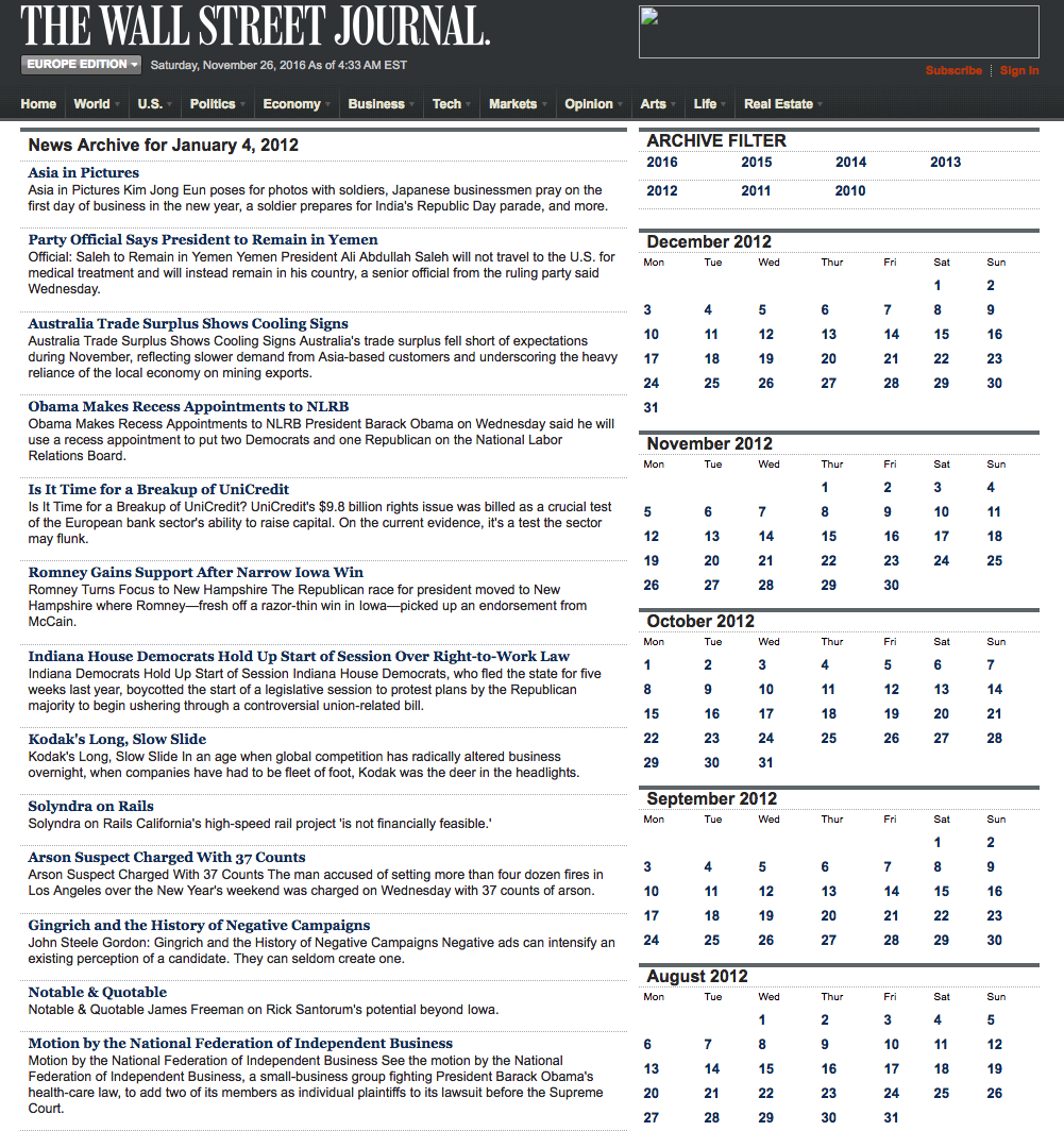
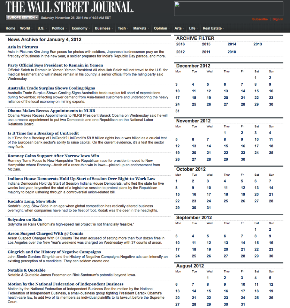
We are going to access the Journal’s online archive, which presents daily news items in a convenient summary format, an example of which is shown below. The archive runs from the beginning of 2012 through to the current day, providing ample data for analysis. In what follows, I am going to make two important assumptions, neither of which is likely to be 100% accurate – but which will not detract too much from the validity of the research, I hope. The first assumption is that the news items shown in each daily archive were reported prior to the market open at 9:30 AM. This is likely to be true for the great majority of the stories, but there are no doubt important exceptions. Since we intend to treat the news content of each archive as antecedent to the market action during the corresponding trading session, exceptions are likely to introduce an element of look-ahead bias. The second assumption is that the archive for each day is shown in the form in which it would have appeared on the day in question. In reality, there are likely to have been revisions to some of the stories made subsequent to their initial publication. So, here too, we must allow for the possibility of look-ahead bias in the ensuing analysis.

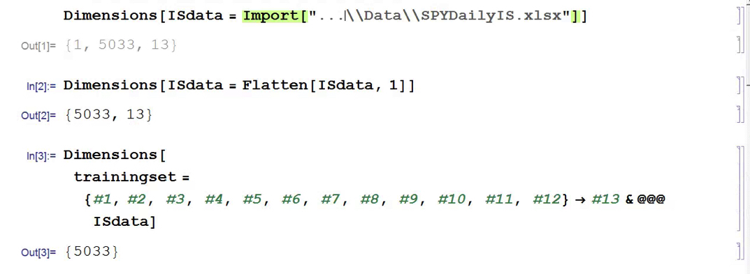
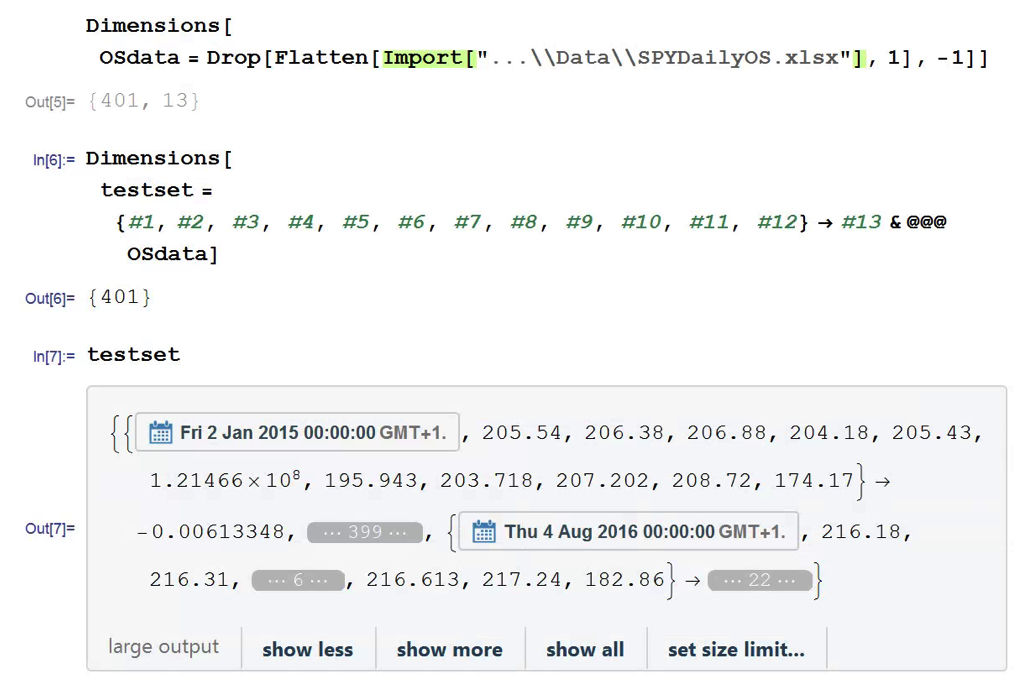
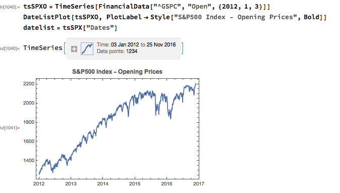
With those caveats out of the way, let’s proceed. We are going to be using broad market data for the S&P 500 index in the analysis to follow, so the first step is to download daily price series for the index. Note that we begin with daily opening prices, since we intend to illustrate the application of news sentiment analysis with a theoretical day-trading strategy that takes positions at the start of each trading session, exiting at market close.

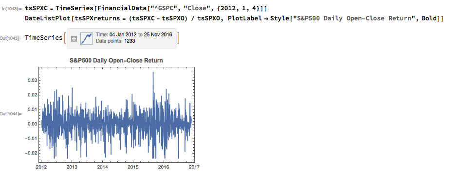
From there we calculate the intraday return in the index, from market open to close, as follows:

Text Analysis & Classification

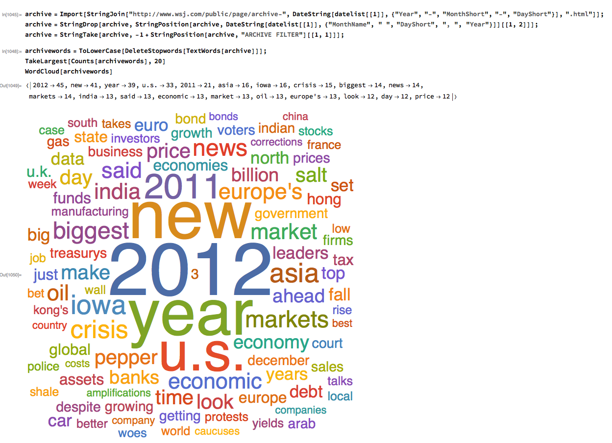
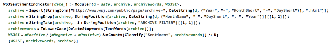
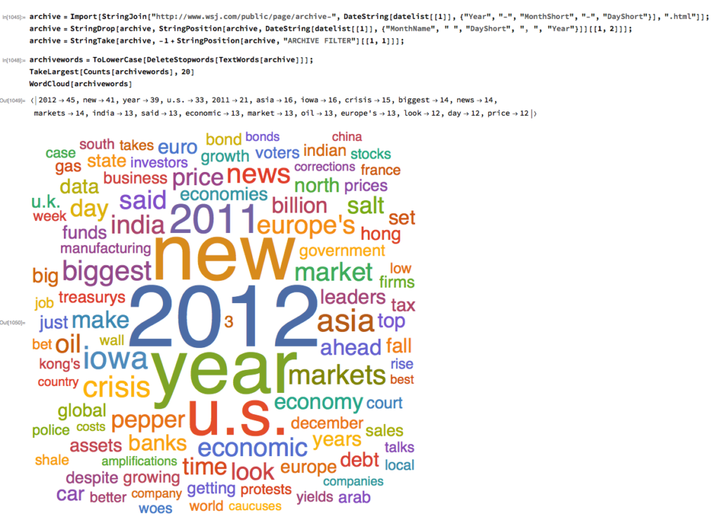
Next we turn to the task of reading the news archive and categorizing its content. Mathematica makes the importation of html pages very straightforward, and we can easily crop the raw text string to exclude page headers and footers. The approach I am going to take is to derive a sentiment indicator based on an analysis of the sentiment of each word in the daily archive. Before we can do that we must first convert the text into individuals words, stripping out standard stop-words such as “the” and “in” and converting all the text to lower case. Naturally one can take this pre-processing a great deal further, by identifying and separating out proper nouns, for example. Once the text processing stage is complete we can quickly summarize the content, for example by looking at the most common words, or by representing the entire archive in the form of a word cloud. Given that we are using the archive for the first business day of 2012, it is perhaps unsurprising that we find that “2012”, “new” and “year” feature so prominently!

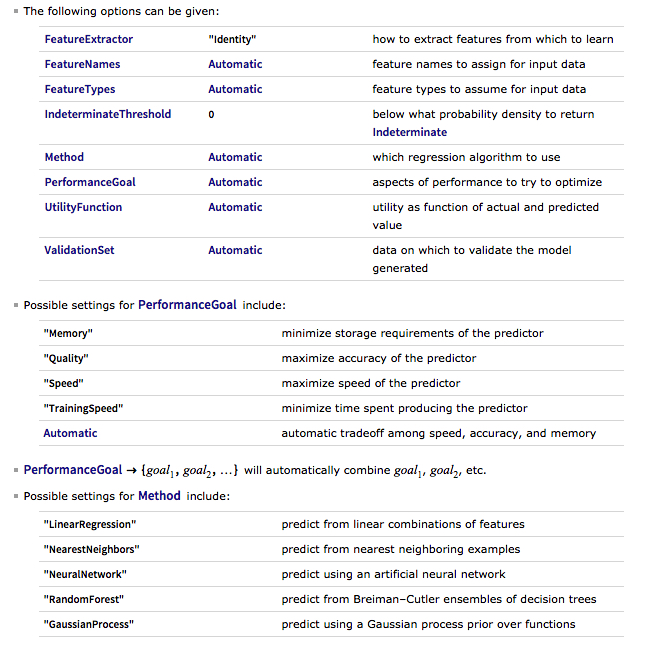
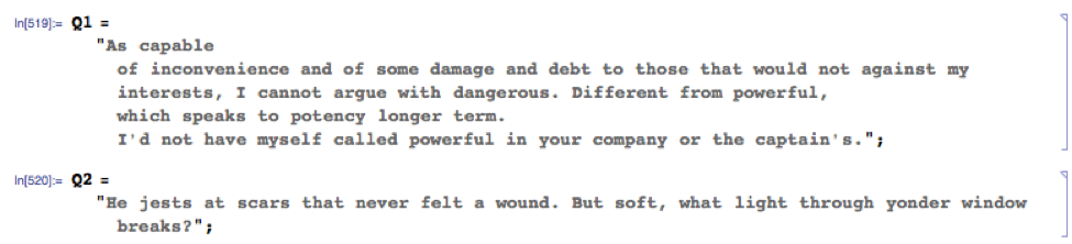
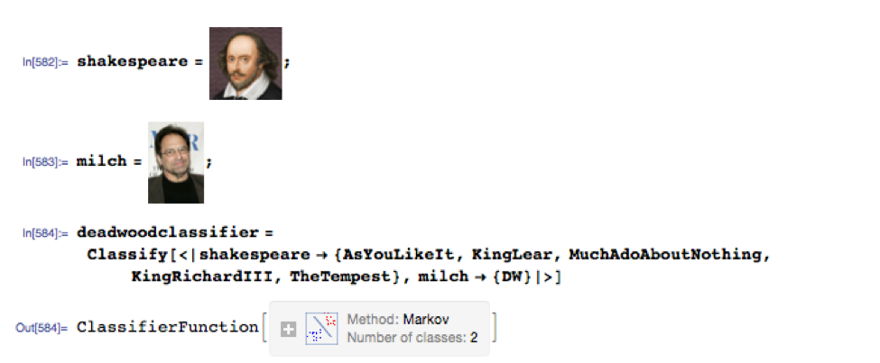
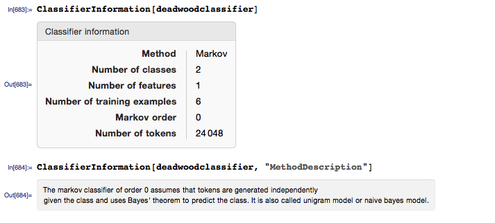
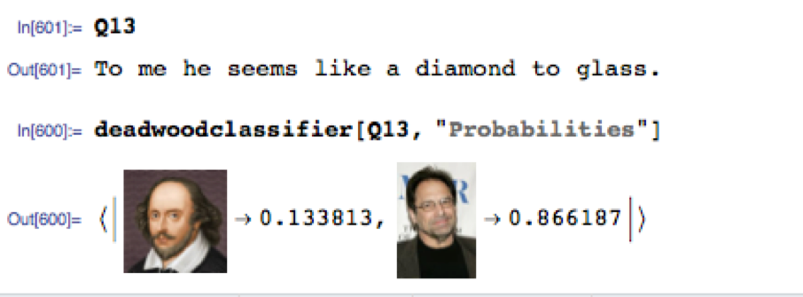
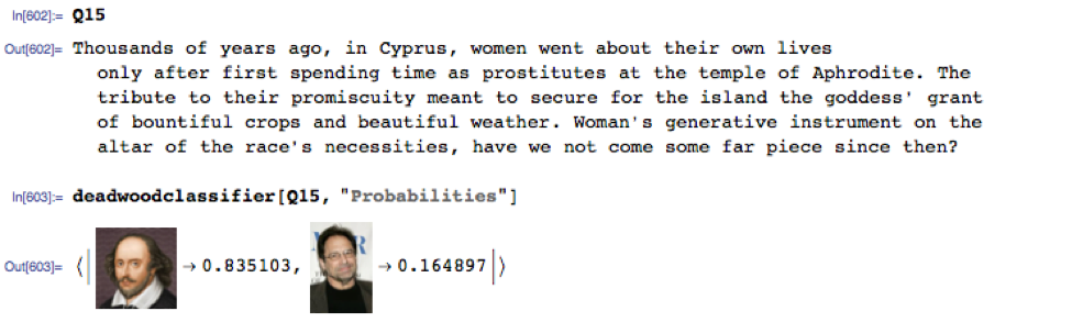
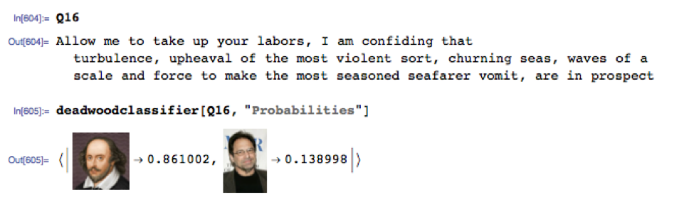
The subject of sentiment analysis is a complex one and I only touch on it here. For those interested in the subject I can recommend The Text Mining Handbook, by Feldman and Sanger, which is a standard work on the topic. Here I am going to employ a machine learning classifier provided with Mathematica 11. It is not terribly sophisticated (or, at least, has not been developed with financial applications especially in mind), but will serve for the purposes of this article. For those unfamiliar with the functionality, the operation of the sentiment classification algorithm is straightforward enough. For instance:

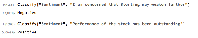
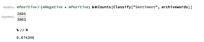
We apply the algorithm to classify each word in the daily news archive and arrive at a sentiment indicator based on the proportion of words that are classified as “positive”. The sentiment reading for the archive for Jan-3, 2012, for example, turns out to be 67.4%:

Sentiment Index Analytics

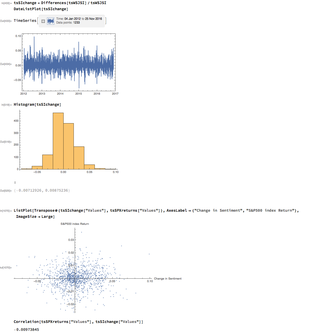
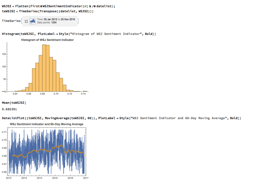
We can automate the process of classifying the entire WSJ archive with just a few lines of code, producing a time series for the daily sentiment indicator, which has an average daily value of 68.5% – the WSJ crowd tends to be bullish, clearly! Note how the 60-day moving average of the indicator rises steadily over the period from 2012 through Q1 2015, then abruptly reverses direction, declining steadily thereafter – even somewhat precipitously towards the end of 2016.

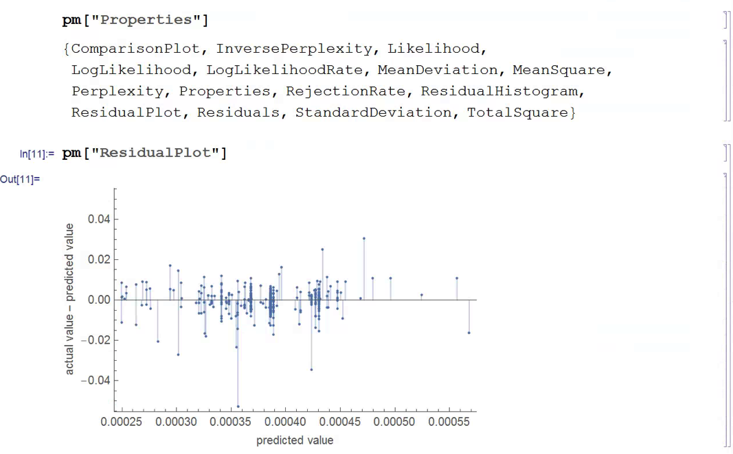
As with most data series in investment research, we are less interested in the level of a variable, such as a stock price, than we are in the changes in level. So the next step is to calculate the daily percentage change in the sentiment indicator and examine the correlation with the corresponding intraday return in the S&P 500 Index. At first glance our sentiment indicator appears to have very little predictive power – the correlation between indicator changes and market returns is negligibly small overall – but we shall later see that this is not the last word.

Conditional Distributions

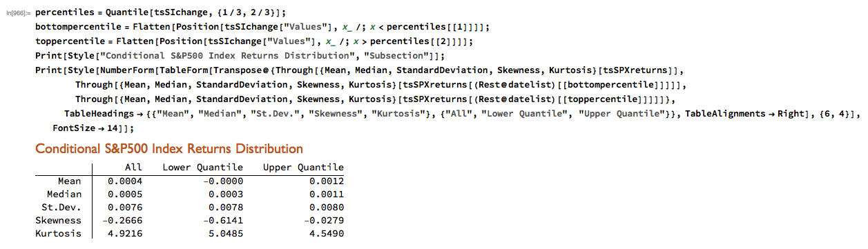
Thus far the results appear discouraging; but as is often the case with this type of analysis we need to look more closely at the conditional distribution of returns. Specifically, we will examine the conditional distribution of S&P 500 Index returns when changes in the sentiment index are in the upper and lower quantiles of the distribution. This will enable us to isolate the impact of changes in market sentiment at times when the swings in sentiment are strongest. In the analysis below, we begin by examining the upper and lower third of the distribution of changes in sentiment:

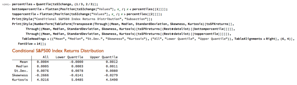
The analysis makes clear that the distribution of S&P 500 Index returns is very different on days when the change in market sentiment is large and positive vs. large and negative. The difference is not just limited to the first moment of the conditional distribution, where the difference in the mean return is large and statistically significant, but also in the third moment. The much larger, negative skewness means that there is a greater likelihood of a large decline in the market on days in which there is a sizable drop in market sentiment, than on days in which sentiment significantly improves. In other words, the influence of market sentiment changes is manifest chiefly through the mean and skewness of the conditional distributions of market returns.

A News Trading Algorithm

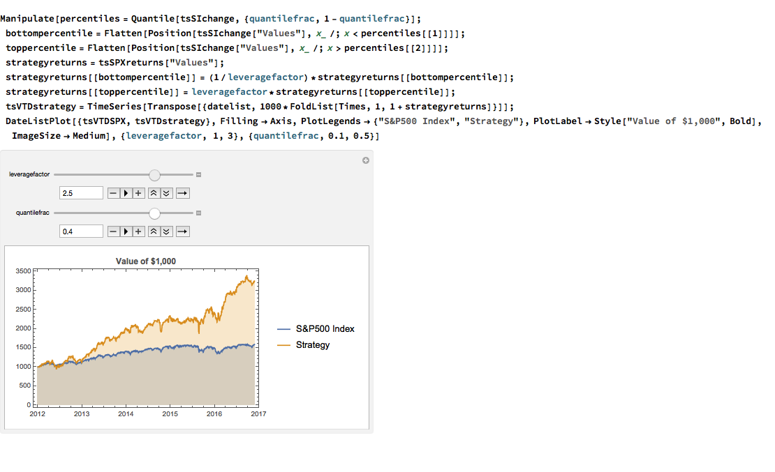
We can capitalize on these effects using a simple trading strategy in which we increase the capital allocated to a long-SPX position on days when market sentiment improves, while reducing exposure on days when market sentiment falls. We increase the allocation by a factor – designated the leverage factor – on days when the change in the sentiment indicator is in the upper 1/3 of the distribution, while reducing the allocation by 1/leveragefactor on days when the change in the sentiment indicator falls in lower 1/3 of the distribution. The allocation on other days is 100%. The analysis runs as follows:

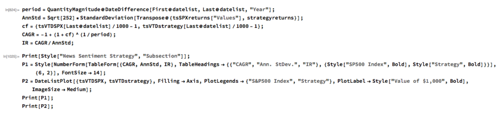
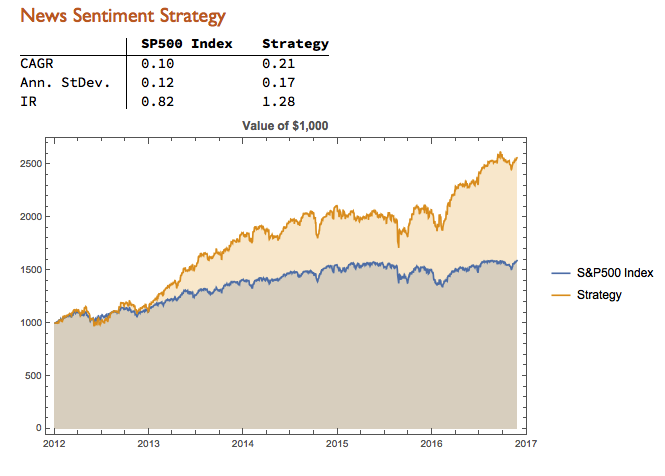
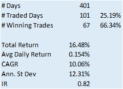
It turns out that, using a leverage factor of 2.0, we can increase the CAGR from 10% to 21% over the period from 2012-2016 using the conditional distribution approach. This performance enhancement comes at a cost, since the annual volatility of the news sentiment strategy is 17% compared to only 12% for the long-only strategy. However, the overall net result is positive, since the risk-adjusted rate of return increases from 0.82 to 1.28.

We can explore the robustness of the result, comparing different quantile selections and leverage factors using Mathematica’s interactive Manipulate function:

Conclusion

We have seen that a simple market sentiment indicator can be created quite easily from publicly available news archives, using a standard machine learning sentiment classification algorithm. A market sentiment algorithm constructed using methods as straightforward as this appears to provide the capability to differentiate the conditional distribution of market returns on days when changes in market sentiment are significantly positive or negative. The differences in the higher moments of the conditional distribution appears to be as significant as the differences in the mean. In principle, we can use the insight provided by the sentiment indicator to enhance a long-only day-trading strategy, increasing leverage and allocation on days when changes to market sentiment are positive and reducing them on days when sentiment declines. The performance enhancements resulting from this approach appear to be significant.

Several caveats apply. The S&P 500 index is not tradable, of course, and it is not uncommon to find trading strategies that produce interesting theoretical results. In practice one would be obliged to implement the strategy using a tradable market proxy, such as a broad market ETF or futures contract. The strategy described here, which enters and exits positions daily, would incur substantial trading costs, that would be further exacerbated by the use of leverage.

Of course there are many other uses one can make of news data, in particular with firm-specific news and sentiment analytics, that fall outside the scope of this article. Hopefully, however, the methodology described here will provide a sign-post towards further, more practically useful research.

September 3, 2019

Dynamic Time Warping

August 27, 2019

Machine Learning Trading Systems

The SPDR S&P 500 ETF (SPY) is one of the widely traded ETF products on the market, with around $200Bn in assets and average turnover of just under 200M shares daily. So the likelihood of being able to develop a money-making trading system using publicly available information might appear to be slim-to-none. So, to give ourselves a fighting chance, we will focus on an attempt to predict the overnight movement in SPY, using data from the prior day’s session.

In addition to the open/high/low and close prices of the preceding day session, we have selected a number of other plausible variables to build out the feature vector we are going to use in our machine learning model:

The daily volume
The previous day’s closing price
The 200-day, 50-day and 10-day moving averages of the closing price
The 252-day high and low prices of the SPY series

We will attempt to build a model that forecasts the overnight return in the ETF, i.e. [O(t+1)-C(t)] / C(t)

In this exercise we use daily data from the beginning of the SPY series up until the end of 2014 to build the model, which we will then test on out-of-sample data running from Jan 2015-Aug 2016. In a high frequency context a considerable amount of time would be spent evaluating, cleaning and normalizing the data. Here we face far fewer problems of that kind. Typically one would standardized the input data to equalize the influence of variables that may be measured on scales of very different orders of magnitude. But in this example all of the input variables, with the exception of volume, are measured on the same scale and so standardization is arguably unnecessary.

First, the in-sample data is loaded and used to create a training set of rules that map the feature vector to the variable of interest, the overnight return:

In Mathematica 10 Wolfram introduced a suite of machine learning algorithms that include regression, nearest neighbor, neural networks and random forests, together with functionality to evaluate and select the best performing machine learning technique. These facilities make it very straightfoward to create a classifier or prediction model using machine learning algorithms, such as this handwriting recognition example:

We create a predictive model on the SPY trainingset, allowing Mathematica to pick the best machine learning algorithm:

There are a number of options for the Predict function that can be used to control the feature selection, algorithm type, performance type and goal, rather than simply accepting the defaults, as we have done here:

Having built our machine learning model, we load the out-of-sample data from Jan 2015 to Aug 2016, and create a test set:

We next create a PredictionMeasurement object, using the Nearest Neighbor model , that can be used for further analysis:

There isn’t much dispersion in the model forecasts, which all have positive value. A common technique in such cases is to subtract the mean from each of the forecasts (and we may also standardize them by dividing by the standard deviation).

The scatterplot of actual vs. forecast overnight returns in SPY now looks like this:

There’s still an obvious lack of dispersion in the forecast values, compared to the actual overnight returns, which we could rectify by standardization. In any event, there appears to be a small, nonlinear relationship between forecast and actual values, which holds out some hope that the model may yet prove useful.

From Forecasting to Trading

There are various methods of deploying a forecasting model in the context of creating a trading system. The simplest route, which we will take here, is to apply a threshold gate and convert the filtered forecasts directly into a trading signal. But other approaches are possible, for example:

Combining the forecasts from multiple models to create a prediction ensemble
Using the forecasts as inputs to a genetic programming model
Feeding the forecasts into the input layer of a neural network model designed specifically to generate trading signals, rather than forecasts

In this example we will create a trading model by applying a simple filter to the forecasts, picking out only those values that exceed a specified threshold. This is a standard trick used to isolate the signal in the model from the background noise. We will accept only the positive signals that exceed the threshold level, creating a long-only trading system. i.e. we ignore forecasts that fall below the threshold level. We buy SPY at the close when the forecast exceeds the threshold and exit any long position at the next day’s open. This strategy produces the following pro-forma results:

Conclusion

The system has some quite attractive features, including a win rate of over 66% and a CAGR of over 10% for the out-of-sample period.

Obviously, this is a very basic illustration: we would want to factor in trading commissions, and the slippage incurred entering and exiting positions in the post- and pre-market periods, which will negatively impact performance, of course. On the other hand, we have barely begun to scratch the surface in terms of the variables that could be considered for inclusion in the feature vector, and which may increase the explanatory power of the model.

In other words, in reality, this is only the beginning of a lengthy and arduous research process. Nonetheless, this simple example should be enough to give the reader a taste of what’s involved in building a predictive trading model using machine learning algorithms.

August 20, 2019

The Swan of Deadwood

Spending 12-14 hours a day managing investors’ money doesn’t leave me a whole lot of time to sit around watching TV. And since I have probably less than 10% of the ad-tolerance of a typical American audience member, I inevitably turn to TiVo, Netflix, or similar, to watch a commercial-free show. Which means that I am inevitably several years behind the cognoscenti of the au-courant. This has its pluses: I avoid a lot of drivel that way.

So it was that I recently tuned in to watch Deadwood, a masterpiece of modern drama written by the talented David Milch, of NYPD Blue fame. The setting of the show is unpromising: a mud-caked camp in South Dakota around the turn of the 19th century that appears to portend yet another formulaic Western featuring liquor, guns, gals and gold and not much else. The first episode appeared at first to confirm my lowest expectations. I struggled through the second. But by the third I was hooked.

What makes Deadwood such a triumph are its finely crafted plots and intricate sub-plots; the many varied and often complex characters, superbly played by Ian McShane (with outstanding performances by Brad Dourif, Powers Boothe, amongst an abundance of others, no less gifted); and, of course, the dialogue.

Yes, the dialogue: hardly the crowning glory of the typical Hollywood Western. And here, to make matters worse, almost every sentence uttered by many of the characters is replete with such shocking profanity that one is eventually numbed into accepting it as normal. But once you get past that, something strange and rather wonderful overtakes you: a sense of being carried along on a river of creative wordsmith-ing that at times eddies, bubbles, plunges and roars its way through scenes that are as comedic, dramatic and action-packed as any I have seen on film. For those who have yet to enjoy the experience, I offer one small morsel:

https://www.youtube.com/watch?v=RdJ4TQ3TnNo

Milch as Shakespeare?

Around the start of Series 2 a rather strange idea occurred to me that, try as I might, I was increasingly unable to suppress as the show progressed: that the writing – some of it at least – was almost Shakespearian in its ingenuity and, at times, lyrical complexity.

Convinced that I had taken leave of my senses I turned to Google and discovered, to my surprise, that there is a whole cottage industry of Deadwood fans who had made the same connection. There is even – if you can imagine it – an online quiz that tests if you are able to identify the source of a number of quotes that might come from the show, or one of the Bard’s many plays. I kid you not:

Intrigued, I took the test and scored around 85%. Not too bad for a science graduate, although I expect most English majors would top 90%-95%. That gave me an idea: could one develop a machine learning algorithm to do the job?

Here’s how it went.

Milch or Shakespeare? – A Machine Learning Classification Algorithm

We start by downloading the text of a representative selection of Shakespeare’s plays, avoiding several of the better-known works from which many of the quotations derive:

For testing purposes, let’s download a sample of classic works by other authors:

Let’s build an initial test classifier, as follows:

It seems to work ok:

So far so good. Let’s import the script for Deadwood series 1-3:

DeadWood = Import[“……../Dropbox/Documents/Deadwood-Seasons-1-3-script.txt”];

Next, let’s import the quotations used in the online test:

etc

We need to remove the relevant quotes from the Deadwood script file used to train the classifier, of course (otherwise it’s cheating!). We will strip an additional 200 characters before the start of each quotation, and 500 characters after each quotation, just for good measure:

and so on….

Now we are ready to build our classifier:

And we can obtain some information about the classifier, as follows:

Let’s see how it performs:

Or, if you prefer tabular form:

The machine learning model scored a total of 19 correct answers out of 23, or 82%.

Fooling the Machine

Let’s take a look as some of the questions the algorithm got wrong.

Quotation no. 13 is challenging, as it comes from Pericles, one of Shakespeare’s lesser-know plays and the idiom appears entirely modern. The classifier assigns an 87% probability of Milch being the author (I got it wrong too).

On Quotation no. 15 the algorithm was just as mistaken, but in the other direction (I got this one right, but only because I recalled the monologue from the episode):

Quotation no.16 strikes me as entirely Shakespearian in form and expression and the classifier thought so too, favoring the Bard by 86% to only 14% for Milch:

Quotation no. 19 had the algorithm fooled completely. It’s a perfect illustration of a typical kind of circumlocution favored by Shakespeare that is imitated so well by Milch’s Deadwood characters:

Conclusion

The model clearly picked up distinguishing characteristics of the two authors’ writings that enabled it to correctly classify 82% of the quotations, quite a high percentage and much better than we would expect to do by tossing a coin, for example. It’s a respectable performance, but I might have hoped for greater accuracy from the model, which scored about the same as I did.

I guess those who see parallels in the writing of William Shakespeare and David Milch may be onto something.

Postscript

The Hollywood Reporter recently published a story entitled

“How the $100 Million ‘NYPD Blue’ Creator Gambled Away His Fortune”.

It’s a fascinating account of the trials and tribulations of this great author, one worthy of Deadwood itself.

A silver lining to this tragic tale, perhaps, is that Milch’s difficulties may prompt him into writing the much-desired Series 4.

One can hope.

September 10, 2018

A Primer on Genetic Programming

Posted by androidMarvin:

Genetic programming is an approach to letting the computer generate its own program code, rather than have a person write the program. It doesn’t specifically “find patterns” or rules within data structures. It starts with a number of randomly-constructed (as long as they are mathematically valid) sample programs, evaluates how close each one is to achieving what the desired result program should achieve, then steadily modifies the best matches to the desired target program in order to improve their match to the desired target; the original random attempts “evolve” towards a better match by natural selection, the best ones being selected to act as the basis for the next generation of attempts.

A tree representing a candidate formula could be represented as follows:

It basically shows the mathematical operations that will be used in the formula, the order in which they are applied, and what values they act on. When the EL Verifier is analysing a statement like

value1 = sin( X ) / a + b * cos( X )

it has to see work out what order the parts of the statement should be evaluated in, which a person sees immediately; effectively, the Verifier constructs the tree diagram above, so that it knows that it has to generate code to make the computer :

take the value of variable X and pass it through a call to the sin() functio
take that result, and divide it by the value of a
take the value of variable X and pass it through a call to the cos() functio
take that result and multiply it by the value of variable
take the result of step 2 and the result of step 4 and add the
that result is the value of Y for the input value of X

Tradestation optimiser would take a single such tree, defining a fixed formula, and attempt to fit it to the data by varying the values of variables a and b. A Genetic Programming optimiser could do the same, but it also has the freedom to change the mathematical operators and the merge points in the tree, and change the shape of the tree to make the formula more or less complex as well; it can adjust both the parameters to the equation and the equation itself in order to evolve it to a better result.

For a mathematical curve fit, a GP optimiser would evaluate each individual tree by applying all the measured X values to the tree’s inputs, compare each output to the measured Y values, and sum a measure of the error over all the data; that sum would be the measure of how well the current tree matches the measure data. The “genetic” part of the name derives from the way it tries to evolve the population of trees its using to find the best.

The main evolution technique is “crossover”. When two parent animals create offspring, each offspring will get part of its DNA from one parent and part from the other; improvement of the species happens if some of the offspring get DNA component combinations that suit the environment better than their parents are suited. The GP optimiser emulates this process by selecting two parent trees, and swapping a section of one of those trees with a section of tree from the other parent, to create two offspring. Eg given parent trees

representing equations

value1 = sin( X )/a + b * cos( X )

and

value1 = cos( X ) / a + b * sin( X )

the offspring might be

representing equations

value1 = sin( X )/cos( X ) + b * cos( X )

and

value1 = a / a + b * sin( X )

Those specific changes are unlikely to both be an improvement, but that’s the way with random processes; the changes made aren’t guided by any sort of principle, its just a case of “change something, anything, and see if its any better”.

A secondary change process that can be used is “mutation”, in which something about a single tree is simply changed, not swapped. This is intended to introduce diversity, so that if none of the current trees is a particularly good performer, there’s a chance that something radically better might be brought into the pool.

The push trying to steer the evolution towards a better result comes from deciding which parents are allowed to create offspring. The original idea was that all the current trees were ranked in sorted order of their fitness, the worst ones were removed from the population to be replaced by new offspring, amd the trees that were the best performing are selected to be parents – so the weak die, and the strongest breed, hoping their offspring will be at least as good as the parents.

One reservation I have about a product like Adaptrade Builder is that it doesn’t follow this original pattern. It chooses “a few” (2 by default) trees to be considered as parents, by entering a “tournament” and the best tree in the tournament is selected as a parent. This seems to me to reduce the bias towards breeding strength with strength, but I’m no expert.

Rather than being simply mathematical, Builder seems to generate tests for entry and exit orders. It takes arithmetic and comparison operators for granted, and allows trees to be built from technical indicators rather than mathematical functions like sin() and cos(). So where an EL programmer might write

if average( Close, fast ) crosses above Average( ( High + Low )/2, slow ) and CCI( length ) > overbought then buy

Builder would have a tree

from which an offspring might be generated as :

to use a Buy test

if average( ( High + Low )/2, fast ) crosses above Average( Close, slow ) and CCI( length ) > overbought then buy

The structure of the test to go long has changed, but in a random rather than the guided way a human might do when trying to develop a strategy.