Long-Only Equity Investors
Recently I have been discussing possible areas of collaboration with an RIA contact on LinkedIn, who also happens to be very familiar with the hedge fund world. He outlined the case of a high net worth investor in equities (long only), who wanted to remain invested, but was becoming increasingly concerned about the prospects for a significant market downturn, or even a market crash, similar to those of 2000 or 2008.
I am guessing he is not alone: hardly a day goes by without the publication of yet another article sounding a warning about stretched equity valuations and the dangerously elevated level of the market.
The question put to me was, what could be done to reduce the risk in the investor’s portfolio?
Typically, conservative investors would have simply moved more of their investment portfolio into fixed income securities, but with yields at such low levels this is hardly an attractive option today. Besides, many see the bond market as representing an even more extreme bubble than equities currently.

Hedging Strategies
The problem with traditional hedging mechanisms such as put options, for example, is that they are relatively expensive and can easily reduce annual returns from the overall portfolio by several hundred basis points. Even at current low level of volatility the performance drag is noticeable, since the potential upside in the equity portfolio is also lower than it has been for some time. A further consideration is that many investors are not mandated – or are simply reluctant – to move beyond traditional equity investing into complex ETF products or derivatives.
An equity long/short hedge fund product is one possible solution, but many equity investors are reluctant to consider shorting stocks under any circumstances, even for hedging purposes. And while a short hedge may provide some downside protection it is unlikely to fully safeguard the investor in a crash scenario. Furthermore, the cost of a hedge fund investment is typically greater than for a long-only product, entailing the payment of a performance fee in addition to management fees that are often higher than for standard investment products.
The Ideal Investment Strategy
Given this background, we can say that the ideal investment strategy is one that:
- Invests long-only in equities
- Is inexpensive to implement (reasonable management fees; no performance fees)
- Does not require shorting stocks, or expensive hedging mechanisms such as options
- Makes acceptable returns during both bull and bear markets
- Is likely to produce positive returns in a market crash scenario
A typical buy-and-hold approach is unlikely to meet only the first three requirements, although an argument could be made that a judicious choice of defensive stocks might enable the investment portfolio to generate returns at an “acceptable” level during a downturn (without being prescriptive as to the precise meaning of that term may be). But no buy-and-hold strategy could ever be expected to prosper during times of severe market stress. A more sophisticated approach is required.
Market Timing
Market timing is regarded as a “holy grail” by some quantitative strategists. The idea, simply, is to increase or reduce risk exposure according to the prospects for the overall market. For a very long time the concept has been dismissed as impossible, by definition, given that markets are mostly efficient. But analysts have persisted in the attempt to develop market timing techniques, motivated by the enormous benefits that a viable market timing strategy would bring. And gradually, over time, evidence has accumulated that the market can be timed successfully and profitably. The rate of progress has accelerated in the last decade by the considerable advances in computing power and the development of machine learning algorithms and application of artificial intelligence to investment finance.
I have written several articles on the subject of market timing that the reader might be interested to review (see below). In this article, however, I want to focus firstly on the work on another investment strategist, Blair Hull.
http://jonathankinlay.com/2014/07/how-to-bulletproof-your-portfolio/
http://jonathankinlay.com/2014/07/enhancing-mutual-fund-returns-with-market-timing/
The Hull Tactical Fund
Blair Hull rose to prominence in the 1980’s and 1990’s as the founder of the highly successful quantitative option market making firm, the Hull Trading Company which at one time moved nearly a quarter of the entire daily market volume on some markets, and executed over 7% of the index options traded in the US. The firm was sold to Goldman Sachs at the peak of the equity market in 1999, for a staggering $531 million.
Blair used the capital to establish the Hull family office, Hull Investments, and in 2013 founded an RIA, Hull Tactical Asset Allocation LLC. The firm’s investment thesis is firmly grounded in the theory of market timing, as described in the paper “A Practitioner’s Defense of Return Predictability”, authored by Blair Hull and Xiao Qiao, in which the issues and opportunities of market timing and return predictability are explored.
In 2015 the firm launched The Hull Tactical Fund (NYSE Arca: HTUS), an actively managed ETF that uses quantitative trading model to take long and short positions in ETFs that seek to track the performance of the S&P 500, as well as leveraged ETFs or inverse ETFs that seek to deliver multiples, or the inverse, of the performance of the S&P 500. The goal to achieve long-term growth from investments in the U.S. equity and Treasury markets, independent of market direction.
How well has the Hull Tactical strategy performed? Since the fund takes the form of an ETF its performance is a matter in the public domain and is published on the firm’s web site. I reproduce the results here, which compare the performance of the HTUS ETF relative to the SPDR S&P 500 ETF (NYSE Arca: SPY):
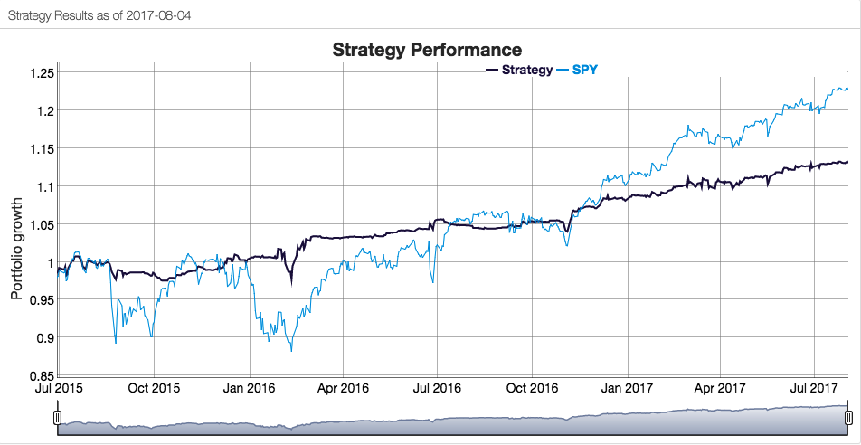
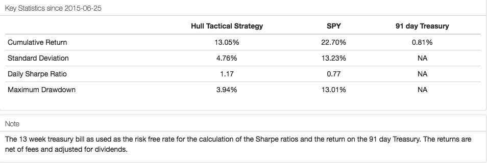
Although the HTUS ETF has underperformed the benchmark SPY ETF since launching in 2015, it has produced a higher rate of return on a risk-adjusted basis, with a Sharpe ratio of 1.17 vs only 0.77 for SPY, as well as a lower drawdown (-3.94% vs. -13.01%). This means that for the same “risk budget” as required to buy and hold SPY, (i.e. an annual volatility of 13.23%), the investor could have achieved a total return of around 36% by using margin funds to leverage his investment in HTUS by a factor of 2.8x.
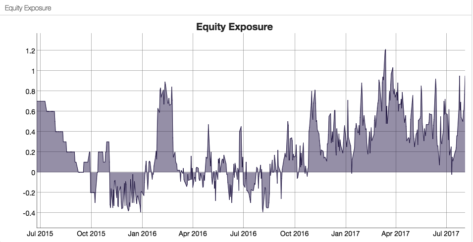
How does the Hull Tactical team achieve these results? While the detailed specifics are proprietary, we know from the background description that market timing (and machine learning concepts) are central to the strategy and this is confirmed by the dynamic level of the fund’s equity exposure over time:
A Long-Only, Crash-Resistant Equity Strategy
A couple of years ago I and my colleagues carried out an investigation of long-only equity strategies as part of a research project. Our primary focus was on index replication, but in the course of our research we came up with a methodology for developing long-only strategies that are highly crash-resistant.
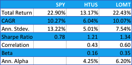
The performance of our Long-Only Market Timing strategy is summarized below and compared with the performance of the HTUS ETF and benchmark SPY ETF (all results are net of fees). Over the period from inception of the HTUS ETF, our LOMT strategy produced a higher total return than HTUS (22.43% vs. 13.17%), higher CAGR (10.07% vs. 6.04%), higher risk adjusted returns (Sharpe Ratio 1.34 vs 1.21) and larger annual alpha (6.20% vs 4.25%). In broad terms, over this period the LOMT strategy produced approximately the same overall return as the benchmark SPY ETF, but with a little over half the annual volatility.

Application of Artificial Intelligence to Market Timing
Like the HTUS ETF, our LOMT strategy operates with very low fees, comparable to an ETF product rather than a hedge fund (1% management fee, no performance fees). Again, like the HTUS ETF our LOMT products makes no use of leverage. However, unlike HTUS it avoids complicated (and expensive) inverse or leveraged ETF products and instead invests only in two assets – the SPY ETF and 91-day US Treasury Bills. In other words, the LOMT strategy is a pure market timing strategy, moving capital between the SPY ETF and Treasury Bills depending on its forecast of future market performance. These forecasts are derived from machine learning algorithms that are specifically tuned to minimize the downside risk in the investment portfolio. This not only makes strategy returns less volatile, but also ensures that the strategy is very robust to market downturns.
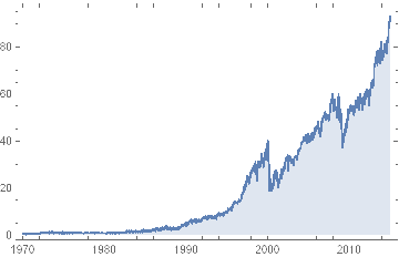
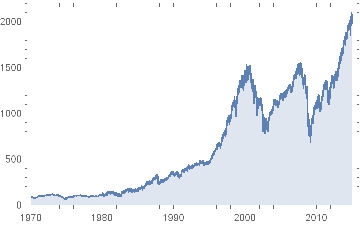
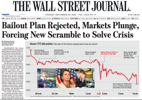
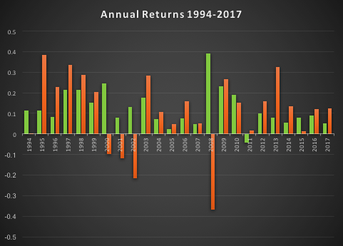
In fact, even better than that, not only does the LOMT strategy tend to avoid large losses during periods of market stress, it is capable of capitalizing on the opportunities that more volatile market conditions offer. Looking at the compounded returns (net of fees) over the period from 1994 (the inception of the SPY ETF) we see that the LOMT strategy produces almost double the total profit of the SPY ETF, despite several years in which it underperforms the benchmark. The reason is clear from the charts: during the periods 2000-2002 and again in 2008, when the market crashed and returns in the SPY ETF were substantially negative, the LOMT strategy managed to produce positive returns. In fact, the banking crisis of 2008 provided an exceptional opportunity for the LOMT strategy, which in that year managed to produce a return nearing +40% at a time when the SPY ETF fell by almost the same amount!

Long Volatility Strategies
I recall having a conversation with Nassim Taleb, of Black Swan fame, about his Empirica fund around the time of its launch in the early 2000’s. He explained that his analysis had shown that volatility was often underpriced due to an under-estimation of tail risk, which the fund would seek to exploit by purchasing cheap out-of-the-money options. My response was that this struck me a great idea for an insurance product, but not a hedge fund – his investors, I explained, were going to hate seeing month after month of negative returns and would flee the fund. By the time the big event occurred there wouldn’t be sufficient AUM remaining to make up the shortfall. And so it proved.
A similar problem arises from most long-volatility strategies, whether constructed using options, futures or volatility ETFs: the combination of premium decay and/or negative carry typically produces continuing losses that are very difficult for the investor to endure.
Conclusion
What investors have been seeking is a strategy that can yield positive returns during normal market conditions while at the same time offering protection against the kind of market gyrations that typically decimate several years of returns from investment portfolios, such as we saw after the market crashes in 2000 and 2008. With the new breed of long-only strategies now being developed using machine learning algorithms, it appears that investors finally have an opportunity to get what they always wanted, at a reasonable price.
And just in time, if the prognostications of the doom-mongers turn out to be correct.
Contact Hull Tactical
Contact Systematic Strategies