Volatility Forecasting in Emerging Markets

The great majority of empirical studies have focused on asset markets in the US and other developed economies.   The purpose of this research is to determine to what extent the findings of other researchers in relation to the characteristics of asset volatility in developed economies applies also to emerging markets.  The important characteristics observed in asset volatility that we wish to identify and examine in emerging markets include clustering, (the tendency for periodic regimes of high or low volatility) long memory, asymmetry, and correlation with the underlying returns process.  The extent to which such behaviors are present in emerging markets will serve to confirm or refute the conjecture that they are universal and not just the product of some factors specific to the intensely scrutinized, and widely traded developed markets.

The ten emerging markets we consider comprise equity markets in Australia, Hong Kong, Indonesia, Malaysia, New Zealand, Philippines, Singapore, South Korea, Sri Lanka and Taiwan focusing on the major market indices for those markets.   After analyzing the characteristics of index volatility for these indices, the research goes on to develop single- and two-factor REGARCH models in the form by Alizadeh, Brandt and Diebold (2002).

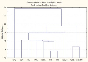
Cluster Analysis of Volatility
Processes for Ten Emerging Market Indices

The research confirms the presence of a number of typical characteristics of volatility processes for emerging markets that have previously been identified in empirical research conducted in developed markets.  These characteristics include volatility clustering, long memory, and asymmetry.   There appears to be strong evidence of a region-wide regime shift in volatility processes during the Asian crises in 1997, and a less prevalent regime shift in September 2001. We find evidence from multivariate analysis that the sample separates into two distinct groups:  a lower volatility group comprising the Australian and New Zealand indices and a higher volatility group comprising the majority of the other indices.

SSALGOTRADING AD

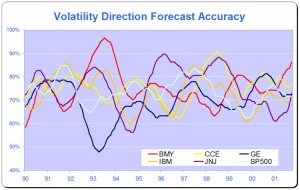
Models developed within the single- and two-factor REGARCH framework of Alizadeh, Brandt and Diebold (2002) provide a good fit for many of the volatility series and in many cases have performance characteristics that compare favorably with other classes of models with high R-squares, low MAPE and direction prediction accuracy of 70% or more.   On the debit side, many of the models demonstrate considerable variation in explanatory power over time, often associated with regime shifts or major market events, and this is typically accompanied by some model parameter drift and/or instability.

Single equation ARFIMA-GARCH models appear to be a robust and reliable framework for modeling asset volatility processes, as they are capable of capturing both the short- and long-memory effects in the volatility processes, as well as GARCH effects in the kurtosis process.   The available procedures for estimating the degree of fractional integration in the volatility processes produce estimates that appear to vary widely for processes which include both short- and long- memory effects, but the overall conclusion is that long memory effects are at least as important as they are for volatility processes in developed markets.  Simple extensions to the single-equation models, which include regressor lags of related volatility series, add significant explanatory power to the models and suggest the existence of Granger-causality relationships between processes.

Extending the modeling procedures into the realm of models which incorporate systems of equations provides evidence of two-way Granger causality between certain of the volatility processes and suggests that are fractionally cointegrated, a finding shared with parallel studies of volatility processes in developed markets.

Download paper here.
Range-Based EGARCH Option Pricing Models (REGARCH)

The research in this post and the related paper on Range Based EGARCH Option pricing Models is focused on the innovative range-based volatility models introduced in Alizadeh, Brandt, and Diebold (2002) (hereafter ABD).  We develop new option pricing models using multi-factor diffusion approximations couched within this theoretical framework and examine their properties in comparison with the traditional Black-Scholes model.

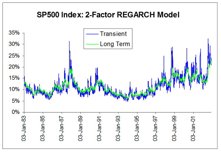
The two-factor version of the model, which I have applied successfully in various option arbitrage strategies, encapsulates the intuively appealing idea of a trending long term mean volatility process, around which oscillates a mean-reverting, transient volatility process.  The option pricing model also incorporates asymmetry/leverage effects and well as correlation effects between the asset return and volatility processes, which results in a volatility skew.

The core concept behind Range-Based Exponential GARCH model is Log-Range estimator discussed in an earlier post on volatility metrics, which contains a lengthy exposition of various volatility estimators and their properties. (Incidentally, for those of you who requested a copy of my paper on Estimating Historical Volatility, I have updated the post to include a link to the pdf).

SSALGOTRADING AD

We assume that the log stock price s follows a drift-less Brownian motion ds = sdW. The volatility of daily log returns, denoted h= s/sqrt(252), is assumed constant within each day, at ht from the beginning to the end of day t, but is allowed to change from one day to the next, from ht at the end of day t to ht+1 at the beginning of day t+1.  Under these assumptions, ABD show that the log range, defined as:

is to a very good approximation distributed as

where N[m; v] denotes a Gaussian distribution with mean m and variance v. The above equation demonstrates that the log range is a noisy linear proxy of log volatility ln ht.  By contrast, according to the results of Alizadeh, Brandt,and Diebold (2002), the log absolute return has a mean of 0.64 + ln ht and a variance of 1.11. However, the distribution of the log absolute return is far from Gaussian.  The fact that both the log range and the log absolute return are linear log volatility proxies (with the same loading of one), but that the standard deviation of the log range is about one-quarter of the standard deviation of the log absolute return, makes clear that the range is a much more informative volatility proxy. It also makes sense of the finding of Andersen and Bollerslev (1998) that the daily range has approximately the same informational content as sampling intra-daily returns every four hours.

Except for the model of Chou (2001), GARCH-type volatility models rely on squared or absolute returns (which have the same information content) to capture variation in the conditional volatility ht. Since the range is a more informative volatility proxy, it makes sense to consider range-based GARCH models, in which the range is used in place of squared or absolute returns to capture variation in the conditional volatility. This is particularly true for the EGARCH framework of Nelson (1990), which describes the dynamics of log volatility (of which the log range is a linear proxy).

ABD consider variants of the EGARCH framework introduced by Nelson (1990). In general, an EGARCH(1,1) model performs comparably to the GARCH(1,1) model of Bollerslev (1987).  However, for stock indices the in-sample evidence reported by Hentschel (1995) and the forecasting performance presented by Pagan and Schwert (1990) show a slight superiority of the EGARCH specification. One reason for this superiority is that EGARCH models can accommodate asymmetric volatility (often called the “leverage effect,” which refers to one of the explanations of asymmetric volatility), where increases in volatility are associated more often with large negative returns than with equally large positive returns.

The one-factor range-based model (REGARCH 1)  takes the form:

where the returns process Rt is conditionally Gaussian: Rt ~ N[0, ht2]

and the process innovation is defined as the standardized deviation of the log range from its expected value:

Following Engle and Lee (1999), ABD also consider multi-factor volatility models.  In particular, for a two-factor range-based EGARCH model (REGARCH2), the conditional volatility dynamics) are as follows:

and

where ln qt can be interpreted as a slowly-moving stochastic mean around which log volatility  ln ht makes large but transient deviations (with a process determined by the parameters kh, fh and dh).

The parameters q, kq, fq and dq determine the long-run mean, sensitivity of the long run mean to lagged absolute returns, and the asymmetry of absolute return sensitivity respectively.

The intuition is that when the lagged absolute return is large (small) relative to the lagged level of volatility, volatility is likely to have experienced a positive (negative) innovation. Unfortunately, as we explained above, the absolute return is a rather noisy proxy of volatility, suggesting that a substantial part of the volatility variation in GARCH-type models is driven by proxy noise as opposed to true information about volatility. In other words, the noise in the volatility proxy introduces noise in the implied volatility process. In a volatility forecasting context, this noise in the implied volatility process deteriorates the quality of the forecasts through less precise parameter estimates and, more importantly, through less precise estimates of the current level of volatility to which the forecasts are anchored.

read more

2-Factor REGARCH Model for the S&P500 Index

Modeling Asset Volatility

I am planning a series of posts on the subject of asset volatility and option pricing and thought I would begin with a survey of some of the central ideas. The attached presentation on Modeling Asset Volatility sets out the foundation for a number of key concepts and the basis for the research to follow.

Perhaps the most important feature of volatility is that it is stochastic rather than constant, as envisioned in the Black Scholes framework.  The presentation addresses this issue by identifying some of the chief stylized facts about volatility processes and how they can be modelled.  Certain characteristics of volatility are well known to most analysts, such as, for instance, its tendency to “cluster” in periods of higher and lower volatility.  However, there are many other typical features that are less often rehearsed and these too are examined in the presentation.

Long Memory
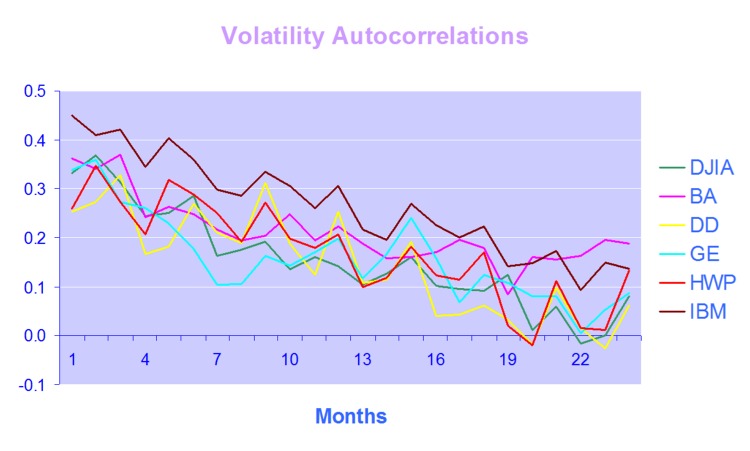
For example, while it is true that GARCH models do a fine job of modeling the clustering effect  they typically fail to capture one of the most important features of volatility processes – long term serial autocorrelation.  In the typical GARCH model autocorrelations die away approximately exponentially, and historical events are seen to have little influence on the behaviour of the process very far into the future.  In volatility processes that is typically not the case, however:  autocorrelations die away very slowly and historical events may continue to affect the process many weeks, months or even years ahead.

Volatility Direction Prediction Accuracy

There are two immediate and very important consequences of this feature.  The first is that volatility processes will tend to trend over long periods – a characteristic of Black Noise or Fractionally Integrated processes, compared to the White Noise behavior that typically characterizes asset return processes.  Secondly, and again in contrast with asset return processes, volatility processes are inherently predictable, being conditioned to a significant degree on past behavior.  The presentation considers the fractional integration frameworks as a basis for modeling and forecasting volatility.

Mean Reversion vs. Momentum
A puzzling feature of much of the literature on volatility is that it tends to stress the mean-reverting behavior of volatility processes.  This appears to contradict the finding that volatility behaves as a reinforcing process, whose long-term serial autocorrelations create a tendency to trend.  This leads to one of the most important findings about asset processes in general, and volatility process in particular: i.e. that the assets processes are simultaneously trending and mean-reverting.  One way to understand this is to think of volatility, not as a single process, but as the superposition of two processes:  a long term process in the mean, which tends to reinforce and trend, around which there operates a second, transient process that has a tendency to produce short term spikes in volatility that decay very quickly.  In other words, a transient, mean reverting processes inter-linked with a momentum process in the mean.  The presentation discusses two-factor modeling concepts along these lines, and about which I will have more to say later.

SSALGOTRADING AD

Cointegration
One of the most striking developments in econometrics over the last thirty years, cointegration is now a principal weapon of choice routinely used by quantitative analysts to address research issues ranging from statistical arbitrage to portfolio construction and asset allocation.  Back in the late 1990’s I and a handful of other researchers realized that volatility processes exhibited very powerful cointegration tendencies that could be harnessed to create long-short volatility strategies, mirroring the approach much beloved by equity hedge fund managers.  In fact, this modeling technique provided the basis for the Caissa Capital volatility fund, which I founded in 2002.  The presentation examines characteristics of multivariate volatility processes and some of the ideas that have been proposed to model them, such as FIGARCH (fractionally-integrated GARCH).

Dispersion Dynamics
Finally, one topic that is not considered in the presentation, but on which I have spent much research effort in recent years, is the behavior of cross-sectional volatility processes, which I like to term dispersion.  It turns out that, like its univariate cousin, dispersion displays certain characteristics that in principle make it highly forecastable.  Given an appropriate model of dispersion dynamics, the question then becomes how to monetize efficiently the insight that such a model offers.  Again, I will have much more to say on this subject, in future.