In this post I want to discuss ways to make use of signals from relevant market indices in your trading. These signals can add value regardless of whether you trade algorithmically or manually. The techniques described here are one of the most widely applicable in the quantitative analyst’s arsenal.
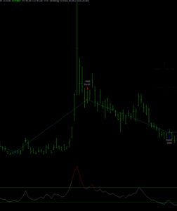
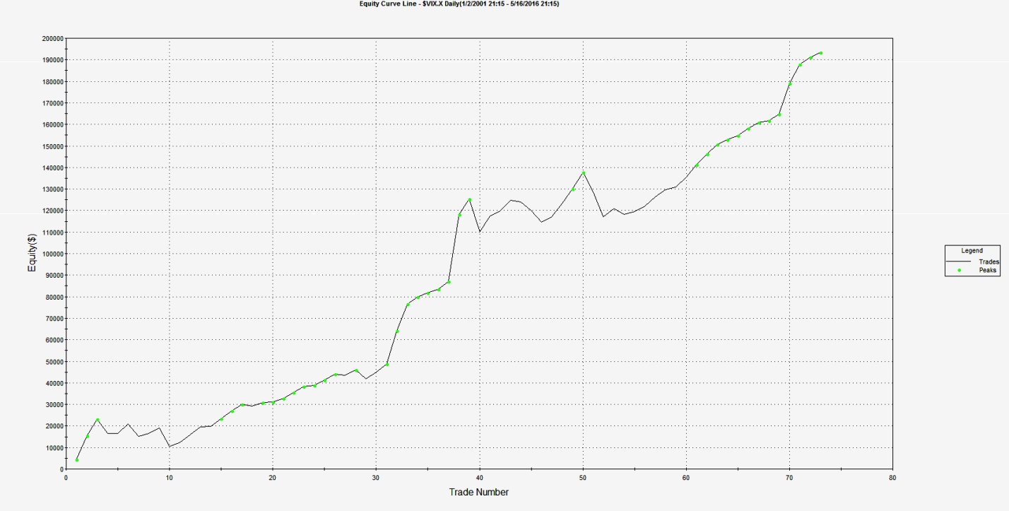
Let’s motivate the discussion by looking an example of a simple trading system trading the VIX on weekly bars. Performance results for the system are summarized in the chart and table below. The system outperforms the buy and hold return by a substantial margin, with a profit factor of over 3 and a win rate exceeding 82%. What’s not to like?
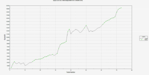
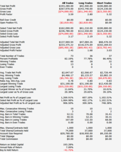
Well, for one thing, this isn’t really a trading system – because the VIX Index itself isn’t tradable. So the performance results are purely notional (and, if you didn’t already notice, no slippage or commission is included).
It is very easy to build high-performing trading system in indices – because they are not traded products, index prices are often stale and tend to “follow” the price action in the equivalent traded market.
This particular system for the VIX Index took me less than ten minutes to develop and comprises only a few lines of code. The system makes use of a simple RSI indicator to decide when to buy or sell the index. I optimized the indicator parameters (separately for long and short) over the period to 2012, and tested it out-of-sample on the data from 2013-2016.
inputs:
Price( Close ) ,
Length( 14 ) ,
OverSold( 30 ) ;
variables:
RSIValue( 0 );
RSIValue = RSI( Price, Length );
if CurrentBar > 1 and RSIValue crosses over OverSold then
Buy ( !( “RsiLE” ) ) next bar at market;
.
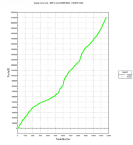
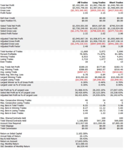
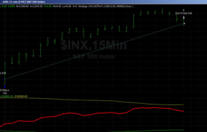
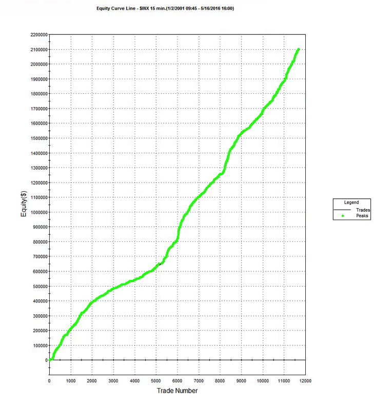
The daily system I built for the S&P 500 Index is a little more sophisticated than the VIX model, and produces the following results.
Using Index Trading Systems
We have seen that its trivially easy to build profitable trading systems for index products. But since they can’t be traded, what’s the point?
The analyst might be tempted by the idea of using the signals generated by an index trading system to trade a corresponding market, such as VIX or eMini futures. However, this approach is certain to fail. Index prices lag the prices of equivalent futures products, where traders first monetize their view on the market. So using an index strategy directly to trade a cash or futures market would be like trying to trade using prices delayed by a few seconds, or minutes – a recipe for losing money.

Nor is it likely that a trading system developed for an index product will generalize to a traded market. What I mean by this is that if you were to take an index strategy, such as the VIX RSI strategy, transfer it to VIX futures and tweak the parameters in the hope of producing a profitable system, you are likely to be disappointed. As I have shown, you can produce a profitable index trading system using the simplest and most antiquated trading concepts (such as the RSI index) that long ago ceased to offer any predictive value in actual traded markets. Index markets are actually inefficient – the prices of index products often fail to fully reflect all relevant, available information in a timely way. Such simple inefficiencies are easily revealed by indicators such as moving averages. Traded markets, by contrast, are highly efficient and, with the exception of HFT, it is going to take a great deal more than a simple moving average to provide insight into the few inefficiencies that do arise.

Strategies in index products are best thought of, not as trading strategies, but rather as a means of providing broad guidance as to the general condition of the market and its likely direction over the longer term. To take the VIX index strategy as an example, you can see that each “trade” spans several weeks. So one might regard a “buy” signal from the VIX index system as an indication that volatility is expected to rise over the next month or two. A trader might use that information to lean on the side of being long volatility, perhaps even avoiding any short volatility positions altogether for the next several weeks. Following the model’s guidance in that way would would certainly have helped many equity and volatility traders during the market sell off during August 2015, for example:
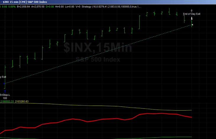
The S&P 500 Index model is one I use to provide guidance as to market conditions for the current trading day. It is a useful input to my thinking as to how aggressive I want my trading models to be during the upcoming session. If the index model suggests a positive tone to the market, with muted volatility, I might be inclined to take a more aggressive stance. If the model starts trading to the short side, however, I am likely to want to be much more cautious. Yesterday (May 16, 2016), for example, the index model took an early long trade, providing confirmation of the positive tenor to the market and encouraging me to trade volatility to the short side more aggressively.
In general, I would tend to classify index trading systems as “decision support” tools that provide a means of shading opinion on the market, or perhaps providing a means of calibrating trading models to the anticipated market conditions. However, they can be used in a more direct way, short of actual trading. For example, one of our volatility trading systems uses the trading signals from a trading system designed for the VVIX volatility-of-volatility index. Another approach is to use the signals from an index trading system as an indicator of the market regime in a regime switching model.
Designing Index Trading Models
Whereas it is profitability that is typically the primary design criterion for an actual trading system, given the purpose of an index trading system there are other criteria that are at least as important.
It should be obvious from these few illustrations that you want to design your index model to trade less frequently than the system you are intending to trade live: if you are swing-trading the eminis on daily bars, it doesn’t help to see 50 trades a day from your index system. What you want is an indication as to whether the market action over the next several days is likely to be positive or negative. This means that, typically, you will design your index system using bar frequencies at least as long as for your live system.
Another way to slow down the signals coming from your index trading system is to design it for very high accuracy – a win rate of 70%, or higher. It is actually quite easy to do this: I have systems that trade the eminis on daily bars that have win rates of over 90%. The trick is simply that you have to be prepared to wait a long time for the trade to come good. For a live system that can often be a problem – no-one like to nurse an underwater position for days or weeks on end. But for an index trading system it matters far less and, in fact, it helps: because you want trading signals over longer horizons than the time intervals you are using in your live trading system.
Since the index system doesn’t have to trade live, it means of course that the usual trading costs and frictions do not apply. The advantage here is that you can come up with concepts for trading systems that would be uneconomic in the real world, but which work perfectly well in the frictionless world of index trading. The downside, however, is that this might lead you to develop index systems that trade far too frequently. So, even though they should not apply, you might seek to introduce trading costs in order to penalize higher frequency trading systems and benefit systems that trade less frequently.
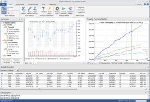
Designing index trading systems in an area in which genetic programming algorithms excel. There are two main reasons for this. Firstly, as I have previously discussed, simple technical indicators of the kind employed by GP modeling systems work well in index markets. Secondly, and more importantly, you can use the GP system to tailor an index trading system to meet the precise criteria you have in mind, such as the % win rate, trading frequency, etc.
An outstanding product that I can highly recommend in this context is Mike Bryant’s Adaptrade Builder. Builder is a superb piece of software whose power and ease of use reflects Mike’s engineering background and systems development expertise.


