Making Money with High Frequency Trading

There is no standard definition of high frequency trading, nor a single type of strategy associated with it. Some strategies generate returns, not by taking any kind of view on market direction, but simply by earning Exchange rebates. In other cases the strategy might try to trade ahead of the news as it flows through the market, from stock to stock (or market to market).  Perhaps the most common and successful approach to HFT is market making, where one tries to earn (some fraction of) the spread by constantly quoting both sides of the market.  In the latter approach, which involves processing vast numbers of order messages and other market data in order to decide whether to quote (or pull a quote), latency is of utmost importance.  I would tend to argue that HFT market making owes its success as much, or more, to computer science than it does to trading or microstructure theory.

By contrast, Systematic Strategies’s approach to HFT has always been model-driven.  We are unable to outgun firms like Citadel or Getco in terms of their speed of execution; so, instead, we focus on developing theoretical models of market behavior, on the assumption that we are more likely to identify a source of true competitive advantage that way.  This leads to slower, less latency-sensitive strategies (the models have to be re-estimated or recomputed in real time), but which may nonetheless trade hundreds of times a day.

A good example is provided by our high frequency scalping strategy in Corn futures, which trades around 100-200 times a day, with a win rate of over 80%.

Corn Monthly PNL EC


One of the most important considerations in engineering a HFT strategy of this kind is to identify a suitable bar frequency.  We find that our approach works best using data at frequencies of 1-5 minutes, trading at latencies of around 1 millisec, whereas other firms are reacting to data tick-by-tick, with latencies measured in microseconds.

Often strategies are built using only data derived from with a single market, based on indicators involving price action, pattern trading rules, volume or volatility signals.  In other cases, however, signals are derived from other, related markets: the VXX-ES-TY complex would be a typical example of this kind of inter-market approach.

SSALGOTRADING AD

When we build strategies we often start by using a simple retail platform like TradeStation or MultiCharts.  We know that if the strategy can make money on a platform with retail levels of order and market data latency (and commission rates), then it should perform well when we transfer it to a production environment, with much lower latencies and costs.  We might be able to trade only 1-2 contracts in TradeStation, but in production we might aim to scale that up to 10-15 contract per trade, or more, depending on liquidity.  For that reason we prefer to trade only intraday, when market liquidity is deepest; but we often find sufficient levels of liquidity to make trading worthwhile 1-2 hours before the open of the day session.

Generally, while we look for outside money for our lower frequency hedge fund strategies, we tend not to do so for our HFT strategies.  After all, what’s the point?  Each strategy has limited capacity and typically requires no more than a $100,000 account, at most.  And besides, with Sharpe Ratios that are typically in double-digits, it’s usually in our economic interest to use all of the capacity ourselves.  Nor do we tend to license strategies to other trading firms.  Again, why would we?  If the strategies work, we can earn far more from trading rather than licensing them.

We have, occasionally, developed strategies for other firms for markets in which we have no interest (the KOSPI springs to mind).  But these cases tend to be the exception, rather than the rule.

Why do Investors Invest in Venture Capital Funds?

 
Too Cool for School?

Startups and Venture Capital are red hot right now. And very cool. If that isn’t a contradiction. Perusing the Business Insider list of “The 38 coolest startups in Silicon Valley”, one is struck by the sheer ingenuity of some ideas. And the total stupidity of others.

Innovation is hard. I have been doing for over 30 years in systematic trading and it never gets any easier. Ideas with great theoretical underpinnings sometimes just don’t work. Others look great in backtest, but fail to transition successfully into production. Some strategies work great for a while, then performance fades as market conditions change. What makes innovation so challenging in the arena of investment management is the competition: millions of very smart minds looking at the same data and trying to come up with something new, often using very similar approaches.

Innovation in the real world is just as challenging, but in a different way. It’s easier in the beginning – you have a whole world of possibilities to play with and so it should be less challenging to come up with something new. But innovation is much more difficult than it first appears. If your idea has any value, chances are someone has already thought of it. They may be developing it now. Or they may have tried to develop the concept and found flaws in it that you have yet to discover.

Innovation Is Hard

I have made a few attempts at innovation in the real world. The first was a product called Easypaycard, a concept that a friend of mine came up with at the start of the internet era. The idea was that you could use the card to send money to anyone, anywhere in the world, via the internet, even if they didn’t have a bank account. Aka Paypal. Couldn’t get anyone interested in that idea.bulb

Then there was a product called Web Telemetrics: a microchip that you could place on any object (or person) and track it on an interactive online map, that would provide not only location, but also other readings like temperature, stress and, in the case of a person, heart rate, etc. Bear in mind, this was in 1999, long before Google maps and location services like Apple’s “find my phone”. I thought it was a rather ingenious concept. The VCs didn’t agree – in the final competition they allocated the money to a company selling women’s shirts online. After that I decided to call it quits, for a while.

There matters stood until 2013, when I came up with a consumer electronics product called Adflik. This contained some quite clever circuitry and machine learning algorithms to detect commercials, when it would switch to the next commercial-free station in your playlist of channels. I thought the product concept was great, but I seriously under-estimated the ad-tolerance of the average American. Only one other person agreed with me! Successful product innovation is tough.

You would think that after three total failures I would hang up my boots. It’s not as though my work in investment research is uncreative, or unrewarding. But I find the idea of developing a physical product, or even an electronic product like an iPhone app, compelling.

 Venture Capital Returns

When you ask a venture capitalist about all this, he is likely to respond, rather haughtily, that his business is not about innovation, but rather to produce a return for his investors. Looking at some of the “hottest” startups, however, suggests to me that we are right back where we were in 1999. That gives me serious cause for concern about the returns that VC funds are likely to produce going forward, especially when interest rates start to rise.

For example, the business model for one of these firms is a grocery delivery service: after you have selected your very expensive groceries from Whole Foods, they will shop and deliver your order to you for an extra $3.99. Sounds like a nice idea, but a $2Bn valuation? Ludicrous. That business is going to evaporate in a puff of smoke at the first sign of a recession, or market correction, which could be right around the corner.

So how good are VC’s at producing investment returns? I did a little digging. What I found was that, while in general the VC fund industry is happy to trumpet its returns, it is almost totally silent about the other half of the investment equation: risk. As for something like a Sharpe Ratio – what that?

To answer I dug up some data from Cambridge Associates on their US Venture Capital Index, which measures quarterly pooled end-to-end net returns to Limited Partners. The index data runs from 1981 to Q2 2014, which is plentiful enough to perform a credible analysis on. Here is what I found:

  • CAGR (1981-Q2 2-14) : 13.85%
  • Annual SD: 20.35%
  • Sharpe Ratio: 0.68

Impressive? Not at all. Any half-decent hedge fund should have a Sharpe Ratio of at least 1. Our own Volatility ETF strategy, for example, has a Sharpe of over 3. We are currently running several high frequency strategies with double-digit Sharpe Ratios.

Note that in computing the Sharpe Ratio, I have ignored the risk free rate of return, which at times during the 1980’s was in double digits. So, if anything, the actual risk adjusted performance is likely significantly lower than stated here.

 VC Funds vs Hedge Funds

Why does this matter? Simple – if you gave me a risk budget equivalent to the VC Index, i.e. a standard deviation of 20% per annum, our volatility strategy would have produced a CAGR of over 60%, for the same degree of investment risk. A high frequency strategy operating at the same risk levels would produce returns north of 200% annually!

Of course, just as with hedge funds, the Cambridge Associates index is an “average” of around 1400 VC funds, some of which will have outperformed the benchmark by a significant margin. Still, the aggregate performance is not exactly stellar.

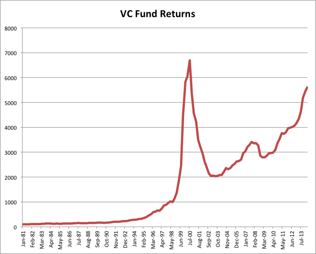
But it gets worse. Look at the chart of the compounded index returns over the period from 1981:

Source: Cambridge Associates

The key point to note is that the index has yet to regain the levels is achieved 15 years ago, before the dot com bust. If VC funds operated high water marks, as most hedge funds do, the overwhelming majority of them would gone out of business many years ago.

So Why Invest in VC Funds?

Given their unimpressive aggregate performance, why do investors invest in VC funds? One answer might lie in the relatively low correlations with other asset classes. For example, over the period from 1981, the correlation between the VC index and the S&P 500 index has averaged only 0.34.

Again, however, if low correlation to the market is the issue, investors can do better by a judicious choice of hedge fund strategy, such as equity market neutral, for example, which typically has a market correlation very close to zero.

Nor is the absolute level of returns a factor: plenty of hedge funds measure their performance in terms of absolute returns. And if investors’ appetite for return is great enough to accommodate a 20% annual volatility, there is no difficulty borrowing at very low margin rates to leverage up the return.

One rational reason for investors’ apparently insatiable appetite for VC funds is capacity: unlike many hedge funds, there is no problem finding investments capable of absorbing multiple $billions, given the global pretensions, rapid burn rates and negligible cash flows of many of these new ventures. But, of course, capacity is only an advantage when the investment itself is sound.

Plowing vast sums into grocery collection services, or online women’s-wear stores, may appear a genius idea to some. But for the rest of us, as the inestimable Lou Reed put it, “other people, they gotta work”.

The Case for Volatility as an Asset Class

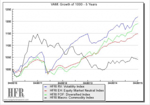
Volatility as an asset class has grown up over the fifteen years since I started my first volatility arbitrage fund in 2000.  Caissa Capital grew to about $400m in assets before I moved on, while several of its rivals have gone on to manage assets in the multiple billions of dollars.  Back then volatility was seen as a niche, esoteric asset class and quite rightly so.  Nonetheless, investors who braved the unknown and stayed the course have been well rewarded: in recent years volatility strategies as an asset class have handily outperformed the indices for global macro, equity market neutral and diversified funds of funds, for example. Fig 1

The Fundamentals of Volatility

It’s worth rehearsing a few of the fundamental features of volatility for those unfamiliar with the territory.

Volatility is Unobservable

Volatility is the ultimate derivative, one whose fair price can never be known, even after the event, since it is intrinsically unobservable.  You can estimate what the volatility of an asset has been over some historical period using, for example, the standard deviation of returns.  But this is only an estimate, one of several possibilities, all of which have shortcomings.  We now know that volatility can be measured with almost arbitrary precision using an integrated volatility estimator (essentially a metric based on high frequency data), but that does not change the essential fact:  our knowledge of volatility is always subject to uncertainty, unlike a stock price, for example.

Volatility Trends

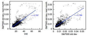
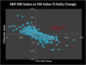
Huge effort is expended in identifying trends in commodity markets and many billions of dollars are invested in trend following CTA strategies (and, equivalently, momentum strategies in equities).  Trend following undoubtedly works, according to academic research, but is also subject to prolonged drawdowns during periods when a trend moderates or reverses. By contrast, volatility always trends.  You can see this from the charts below, which express the relationship between volatility in the S&P 500 index in consecutive months.  The r-square of the regression relationship is one of the largest to be found in economics. Fig 2 And this is a feature of volatility not just in one asset class, such as equities, nor even for all classes of financial assets, but in every time series process for which data exists, including weather and other natural phenomena.  So an investment strategy than seeks to exploit volatility trends is relying upon one of the most consistent features of any asset process we know of (more on this topic in Long Memory and Regime Shifts in Asset Volatility).

Volatility Mean-Reversion and Correlation

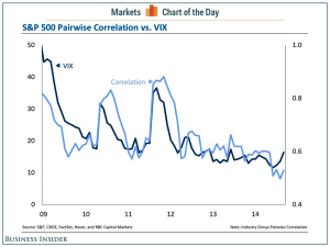
One of the central assumptions behind the ever-popular stat-arb strategies is that the basis between two or more correlated processes is stationary. Consequently, any departure from the long term relationship between such assets will eventually revert to the mean. Mean reversion is also an observed phenomenon in volatility processes.  In fact, the speed of mean reversion (as estimated in, say, an Ornstein-Ulenbeck framework) is typically an order of magnitude larger than for a typical stock-pairs process.  Furthermore, the correlation between one volatility process and another volatility process, or indeed between a volatility process and an asset returns process, tends to rise when markets are stressed (i.e. when volatility increases). Fig 3

Another interesting feature of volatility correlations is that they are often lower than for the corresponding asset returns processes.  One can therefore build a diversified volatility portfolio with far fewer assets that are required for, say, a basket of equities (see Modeling Asset Volatility for more on this topic).

Fig 4   Finally, more sophisticated stat-arb strategies tend to rely on cointegration rather than correlation, because cointegrated series are often driven by some common fundamental factors, rather than purely statistical ones, which may prove temporary (see Developing Statistical Arbitrage Strategies Using Cointegration for more details).  Again, cointegrated relationships tend to be commonplace in the universe of volatility processes and are typically more reliable over the long term than those found in asset return processes.

Volatility Term Structure

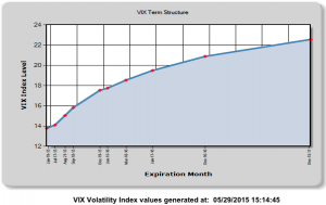
One of the most marked characteristics of the typical asset volatility process its upward sloping term structure.  An example of the typical term structure for futures on the VIX S&P 500 Index volatility index (as at the end of May, 2015), is shown in the chart below. A steeply upward-sloping curve characterizes the term structure of equity volatility around 75% of the time.

Fig 5   Fixed income investors can only dream of such yield in the current ZIRP environment, while f/x traders would have to plunge into the riskiest of currencies to achieve anything comparable in terms of yield differential and hope to be able to mitigate some of the devaluation risk by diversification.

The Volatility of Volatility

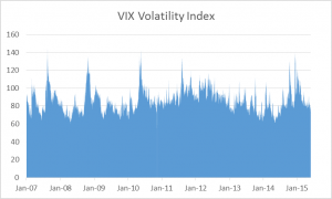
One feature of volatility processes that has been somewhat overlooked is the consistency of the volatility of volatility.  Only on one occasion since 2007 has the VVIX index, which measures the annual volatility of the VIX index, ever fallen below 60.

Fig 6   What this means is that, in trading volatility, you are trading an asset whose annual volatility has hardly ever fallen below 60% and which has often exceeded 100% per year.  Trading opportunities tend to abound when volatility is consistently elevated, as here (and, conversely, the performance of many hedge fund strategies tends to suffer during periods of sustained, low volatility)

SSALGOTRADING AD

Anything You Can Do, I Can Do better

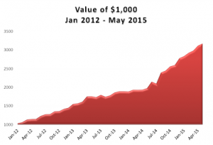
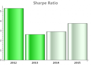
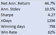
The take-away from all this should be fairly obvious:  almost any strategy you care to name has an equivalent in the volatility space, whether it be volatility long/short, relative value, stat-arb, trend following or carry trading. What is more, because of the inherent characteristics of volatility, all these strategies tend to produce higher levels of performance than their more traditional counterparts. Take as an example our own Volatility ETF strategy, which has produced consistent annual returns of between 30% and 40%, with a Sharpe ratio in excess of 3, since 2012.   VALUE OF $1000

Sharpe

  Monthly Returns


(click to enlarge)

Where does the Alpha Come From?

It is traditional at this stage for managers to point the finger at hedgers as the source of abnormal returns and indeed I will do the same now.   Equity portfolio managers are hardly ignorant of the cost of using options and volatility derivatives to hedge their portfolios; but neither are they likely to be leading experts in the pricing of such derivatives.  And, after all, in a year in which they might be showing a 20% to 30% return, saving a few basis points on the hedge is neither here nor there, compared to the benefits of locking in the performance gains (and fees!). The same applies even when the purpose of using such derivatives is primarily to produce trading returns. Maple Leaf’s George Castrounis puts it this way:

Significant supply/demand imbalances continuously appear in derivative markets. The principal users of options (i.e. pension funds, corporates, mutual funds, insurance companies, retail and hedge funds) trade these instruments to express a view on the direction of the underlying asset rather than to express a view on the volatility of that asset, thus making non-economic volatility decisions. Their decision process may be driven by factors that have nothing to do with volatility levels, such as tax treatment, lockup, voting rights, or cross ownership. This creates opportunities for strategies that trade volatility.

We might also point to another source of potential alpha:  the uncertainty as to what the current level of volatility is, and how it should be priced.  As I have already pointed out, volatility is intrinsically uncertain, being unobservable.  This allows for a disparity of views about its true level, both currently and in future.  Secondly, there is no universal agreement on how volatility should be priced.  This permits at times a wide divergence of views on fair value (to give you some idea of the complexities involved, I would refer you to, for example, Range based EGARCH Option pricing Models). What this means, of course, is that there is a basis for a genuine source of competitive advantage, such as the Caissa Capital fund enjoyed in the early 2000s with its advanced option pricing models. The plethora of volatility products that have emerged over the last decade has only added to the opportunity set.

 Why Hasn’t It Been Done Before?

This was an entirely legitimate question back in the early days of volatility arbitrage. The cost of trading an option book, to say nothing of the complexities of managing the associated risks, were significant disincentives for both managers and investors.  Bid/ask spreads were wide enough to cause significant heads winds for strategies that required aggressive price-taking.  Mangers often had to juggle two sets of risks books, one reflecting the market’s view of the portfolio Greeks, the other the model view.  The task of explaining all this to investors, many of whom had never evaluated volatility strategies previously, was a daunting one.  And then there were the capacity issues:  back in the early 2000s a $400m long/short option portfolio would typically have to run to several hundred names in order to meet liquidity and market impact risk tolerances. Much has changed over the last fifteen years, especially with the advent of the highly popular VIX futures contract and the newer ETF products such as VXX and XIV, whose trading volumes and AUM are growing rapidly.  These developments have exerted strong downward pressure on trading costs, while providing sufficient capacity for at least a dozen volatility funds managing over $1Bn in assets.

Why Hasn’t It Been Done Right Yet?

Again, this question is less apposite than it was ten years ago and since that time there have been a number of success stories in the volatility space. One of the learning points occurred in 2004-2007, when volatility hit the lows for a 20 month period, causing performance to crater in long volatility funds, as well as funds with a volatility neutral mandate. I recall meeting with Nassim Taleb to discuss his Empirica volatility fund prior to that period, at the start of the 2000s.  My advice to him was that, while he had some great ideas, they were better suited to an insurance product rather than a hedge fund.  A long volatility fund might lose money month after month for an entire year, and with it investors and AUM, before seeing the kind of payoff that made such investment torture worthwhile.  And so it proved.

Conversely, stories about managers of short volatility funds showing superb performance, only to blow up spectacularly when volatility eventually explodes, are legion in this field.  One example comes to mind of a fund in Long Beach, CA, whose prime broker I visited with sometime in 2002.  He told me the fund had been producing a rock-steady 30% annual return for several years, and the enthusiasm from investors was off the charts – the fund was managing north of $1Bn by then.  Somewhat crestfallen I asked him how they were producing such spectacular returns.  “They just sell puts in the S&P, 100 points out of the money”, he told me.  I waited, expecting him to continue with details of how the fund managers handled the enormous tail risk.  I waited in vain. They were selling naked put options.  I can only imagine how those guys did when the VIX blew up in 2003 and, if they made it through that, what on earth happened to them in 2008!

Conclusion

The moral is simple:  one cannot afford to be either all-long, or all-short volatility.  The fund must run a long/short book, buying cheap Gamma and selling expensive Theta wherever possible, and changing the net volatility exposure of the portfolio dynamically, to suit current market conditions. It can certainly be done; and with the new volatility products that have emerged in recent years, the opportunities in the volatility space have never looked more promising.

High Frequency Trading Strategies

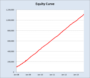
Most investors have probably never seen the P&L of a high frequency trading strategy.  There is a reason for that, of course:  given the typical performance characteristics of a HFT strategy, a trading firm has little need for outside capital.  Besides, HFT strategies can be capacity constrained, a major consideration for institutional investors.  So it is amusing to see the reaction of an investor on encountering the track record of a HFT strategy for the first time.  Accustomed as they are to seeing Sharpe ratios in the range of 0.5-1.5, or perhaps as high as 1.8, if they are lucky, the staggering risk-adjusted returns of a HFT strategy, which often have double-digit Sharpe ratios, are truly mind-boggling.

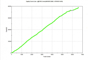
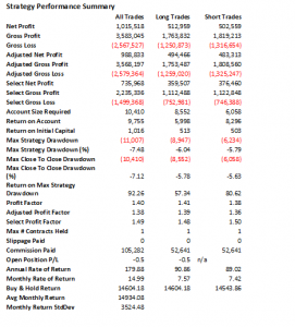
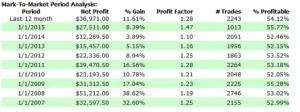
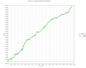
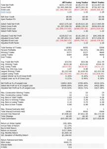
By way of illustration I have attached below the performance record of one such HFT strategy, which trades around 100 times a day in the eMini S&P 500 contract (including the overnight session).  Note that the edge is not that great – averaging 55% profitable trades and profit per contract of around half a tick – these are some of the defining characteristics of HFT trading strategies.  But due to the large number of trades it results in very substantial profits.  At this frequency, trading commissions are very low, typically under $0.1 per contract, compared to $1 – $2 per contract for a retail trader (in fact an HFT firm would typically own or lease exchange seats to minimize such costs).

Fig 2 Fig 3 Fig 4


Hidden from view in the above analysis are the overhead costs associated with implementing such a strategy: the market data feed, execution platform and connectivity capable of handling huge volumes of messages, as well as algo logic to monitor microstructure signals and manage order-book priority.  Without these, the strategy would be impossible to implement profitably.

SSALGOTRADING AD

Scaling things back a little, lets take a look at a day-trading strategy that trades only around 10 times a day, on 15-minute bars.  Although not ultra-high frequency, the strategy nonetheless is sufficiently high frequency to be very latency sensitive. In other words, you would not want to try to implement such a strategy without a high quality market data feed and low-latency trading platform capable of executing at the 1-millisecond level.  It might just be possible to implement a strategy of this kind using TT’s ADL platform, for example.

While the win rate and profit factor are similar to the first strategy, the lower trade frequency allows for a higher trade PL of just over 1 tick, while the equity curve is a lot less smooth reflecting a Sharpe ratio that is “only” around 2.7.

Fig 5 Fig 6 Fig 7


The critical assumption in any HFT strategy is the fill rate.  HFT strategies execute using limit or IOC orders and only a certain percentage of these will ever be filled.  Assuming there is alpha in the signal, the P&L grows in direct proportion to the number of trades, which in turn depends on the fill rate.  A fill rate of 10% to 20% is usually enough to guarantee profitability (depending on the quality of the signal). A low fill rate, such as would typically be seen if one attempted to trade on a retail trading platform, would  destroy the profitability of any HFT strategy.

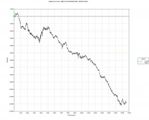
To illustrate this point, we can take a look at the outcome if the above strategy was implemented on a trading platform which resulted in orders being filled only when the market trades through the limit price.  It isn’t a pretty sight.


Fig 8

The moral of the story is:  developing a HFT trading algorithm that contains a viable alpha signal is only half the picture.  The trading infrastructure used to implement such a strategy is no less critical.  Which is why HFT firms spend tens, or hundreds of millions of dollars developing the best infrastructure they can afford.

Designing a Scalable Futures Strategy

I have been working on a higher frequency version of the eMini S&P 500 futures strategy, based on 3-minute bar intervals, which is designed to trade a couple of times a week, with hold periods of 2-3 days.  Even higher frequency strategies are possible, of course, but my estimation is that a hold period of under a week provides the best combination of liquidity and capacity.  Furthermore, the strategy is of low enough frequency that it is not at all latency sensitive – indeed, in the performance analysis below I have assumed that the market must trade through the limit price before the system enters a trade (relaxing the assumption and allowing the system to trade when the market touches the limit price improves the performance).

The other important design criteria are the high % of profitable trades and Kelly f (both over 95%).  This enables the investor to employ money management techniques, such a fixed-fractional allocation for example, in order to scale the trade size up from 1 to 10 contracts, without too great a risk of a major drawdown in realized P&L.

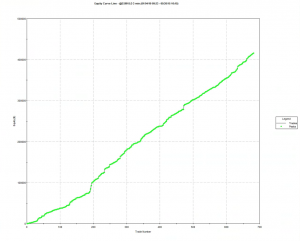
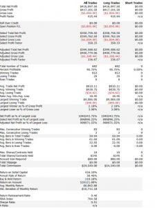
The end result is a strategy that produces profits of $80,000 to $100,000 a year on a 10 contract position, with an annual rate of return of 30% and a Sharpe ratio in excess of 2.0.

Furthermore, of the 682 trades since Jan 2010, only 29 have been losers.

Annual P&L (out of sample)

Annual PL


Equity Curve

EC

Strategy Performance

Perf 1

What’s the Downside?

Everything comes at a price, of course.  Firstly, the strategy is long-only and, by definition, will perform poorly in falling markets, such as we saw in 2008.  That’s a defensible investment thesis, of course – how many $billions are invested in buy and hold strategies? – and, besides, as one commentator remarked, the trick is to develop multiple strategies for different market regimes (although, sensible as that sounds, one is left with the difficulty of correctly identifying the market regime).

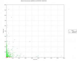
The second drawback is revealed by the trade chart below, which plots the drawdown experienced during each trade.  The great majority of these drawdowns are unrealized, and in most cases the trade recovers to make a profit.  However, there are some very severe cases, such as Sept 2014, when the strategy experienced a drawdown of $85,000 before recovering to make a profit on the trade.  For most investors, the agony of risking an entire year’s P&L just to make a few hundred dollars would be too great.

SSALGOTRADING AD

It should be pointed out that the by the time the drawdown event took place the strategy had already produced many hundreds of thousands of dollars of profit.  So, one could take the view that by that stage the strategy was playing with “house money” and could well afford to take such a risk.

One obvious “solution” to the drawdown problem is to use some kind of stop loss. Unfortunately, the effect is simply to convert an unrealized drawdown into a realized loss.  For some, however, it might be preferable to take a hit of $40,000 or $50,000 once every few years, rather than suffer the  uncertainty of an even larger potential loss.  Either way, despite its many pleasant characteristics, this is not a strategy for investors with weak stomachs!

Trade

Investing in Leveraged ETFs – Theory and Practice

Summary

Leveraged ETFs suffer from decay, or “beta slippage.” Researchers have attempted to exploit this effect by shorting pairs of long and inverse leveraged ETFs.

The results of these strategies look good if you assume continuous compounding, but are often poor when less frequent compounding is assumed.

In reality, the trading losses incurred in rebalancing the portfolio, which requires you to sell low and buy high, overwhelm any benefit from decay, making the strategies unprofitable in practice.

A short levered ETF strategy has similar characteristics to a short straddle option position, with positive Theta and negative Gamma, and will experience periodic, large drawdowns.

It is possible to develop leveraged ETF strategies producing high returns and Sharpe ratios with relative value techniques commonly used in option trading strategies.

SSALGOTRADING AD

Decay in Leveraged ETFs

Leveraged ETFs continue to be much discussed on Seeking Alpha.

One aspect in particular that has caught analysts’ attention is the decay, or “beta slippage” that leveraged ETFs tend to suffer from.

Seeking Alpha contributor Fred Picard in a 2013 article (“What You Need To Know About The Decay Of Leveraged ETFs“) described the effect using the following hypothetical example:

To understand what is beta-slippage, imagine a very volatile asset that goes up 25% one day and down 20% the day after. A perfect double leveraged ETF goes up 50% the first day and down 40% the second day. On the close of the second day, the underlying asset is back to its initial price:

(1 + 0.25) x (1 – 0.2) = 1

And the perfect leveraged ETF?

(1 + 0.5) x (1 – 0.4) = 0.9

Nothing has changed for the underlying asset, and 10% of your money has disappeared. Beta-slippage is not a scam. It is the normal mathematical behavior of a leveraged and rebalanced portfolio. In case you manage a leveraged portfolio and rebalance it on a regular basis, you create your own beta-slippage. The previous example is simple, but beta-slippage is not simple. It cannot be calculated from statistical parameters. It depends on a specific sequence of gains and losses.

Fred goes on to make the point that is the crux of this article, as follows:

At this point, I’m sure that some smart readers have seen an opportunity: if we lose money on the long side, we make a profit on the short side, right?

Shorting Leveraged ETFs

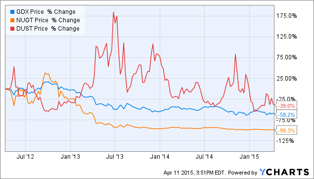
Taking his cue from Fred’s article, Seeking Alpha contributor Stanford Chemist (“Shorting Leveraged ETF Pairs: Easier Said Than Done“) considers the outcome of shorting pairs of leveraged ETFs, including the Market Vectors Gold Miners ETF (NYSEARCA:GDX), the Direxion Daily Gold Miners Bull 3X Shares ETF (NYSEARCA:NUGT) and the Direxion Daily Gold Miners Bear 3X Shares ETF (NYSEARCA:DUST).

His initial finding appears promising:

Therefore, investing $10,000 each into short positions of NUGT and DUST would have generated a profit of $9,830 for NUGT, and $3,900 for DUST, good for an average profit of 68.7% over 3 years, or 22.9% annualized.

At first sight, this appears to a nearly risk-free strategy; after all, you are shorting both the 3X leveraged bull and 3X leveraged bear funds, which should result in a market neutral position. Is there easy money to be made?
Source: Standford Chemist

Not so fast! Stanford Chemist applies the same strategy to another ETF pair, with a very different outcome:

“What if you had instead invested $10,000 each into short positions of the Direxion Russell 1000 Financials Bullish 3X ETF (NYSEARCA:FAS) and the Direxion Russell 1000 Financials Bearish 3X ETF (NYSEARCA:FAZ)?

The $10,000 short position in FAZ would have gained you $8,680. However, this would have been dwarfed by the $28,350 loss that you would have sustained in shorting FAS. In total, you would be down $19,670, which translates into a loss of 196.7% over three years, or 65.6% annualized.

No free lunch there.

The Rebalancing Issue

Stanford Chemist puts his finger on one of the key issues: rebalancing. He explains as follows:

So what happened to the FAS-FAZ pair? Essentially, what transpired was that as the underlying asset XLF increased in value, the two short positions became unbalanced. The losing side (short FAS) ballooned in size, making further losses more severe. On the other hand, the winning side (short FAZ) shrunk, muting the effect of further gains.

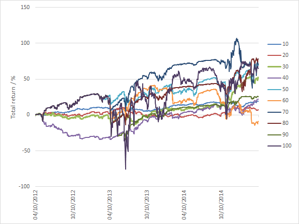
To counteract this effect, the portfolio needs to be rebalanced. Stanford Chemist looks at the implications of rebalancing a short NUGT-DUST portfolio whenever the market value of either ETF deviates by more than N% from its average value, where he considers N% in the range from 10% to 100%, in increments of 10%.

While the annual portfolio return was positive in all but one of these scenarios, there was very considerable variation in the outcomes, with several of the rebalanced portfolios suffering very large drawdowns of as much as 75%:
Source: Stanford Chemist

The author concludes:

The results of the backtest showed that profiting from this strategy is easier said than done. The total return performances of the strategy over the past three years was highly dependent on the rebalancing thresholds chosen. Unfortunately, there was also no clear correlation between the rebalancing period used and the total return performance. Moreover, the total return profiles showed that large drawdowns do occur, meaning that despite being ostensibly “market neutral”, this strategy still bears a significant amount of risk.

Leveraged ETF Pairs – Four Case Studies

Let’s press pause here and review a little financial theory. As you recall, it is possible to express a rate of return in many different ways, depending on how interest is compounded. The most typical case is daily compounding:

R = (Pt – Pt-1) / Pt

Where Pt is the price on day t, and Pt-1 is the price on day t-1, one day prior.

Another commonly used alternative is continuous compounding, also sometimes called log-returns:

R = Ln(Pt) – Ln(Pt-1)

Where Ln(Pt) is the natural log of the price on day t, Pt

When a writer refers to a rate of return, he should make clear what compounding basis the return rate is quoted on, whether continuous, daily, monthly or some other frequency. Usually, however, the compounding basis is clear from the context. Besides, it often doesn’t make a large difference anyway. But with leveraged ETFs, even microscopic differences can produce substantially different outcomes.

I will illustrate the effect of compounding by reference to examples of portfolios comprising short positions in the following representative pairs of leveraged ETFs:

  • Direxion Daily Energy Bull 3X Shares ETF (NYSEARCA:ERX)
  • Direxion Daily Energy Bear 3X Shares ETF (NYSEARCA:ERY)
  • Direxion Daily Gold Miners Bull 3X ETF
  • Direxion Daily Gold Miners Bear 3X ETF
  • Direxion Daily S&P 500 Bull 3X Shares ETF (NYSEARCA:SPXL)
  • Direxion Daily S&P 500 Bear 3X Shares ETF (NYSEARCA:SPXS)
  • Direxion Daily Small Cap Bull 3X ETF (NYSEARCA:TNA)
  • Direxion Daily Small Cap Bear 3X ETF (NYSEARCA:TZA)

The findings in relation to these pairs are mirrored by results for other leveraged ETF pairs.

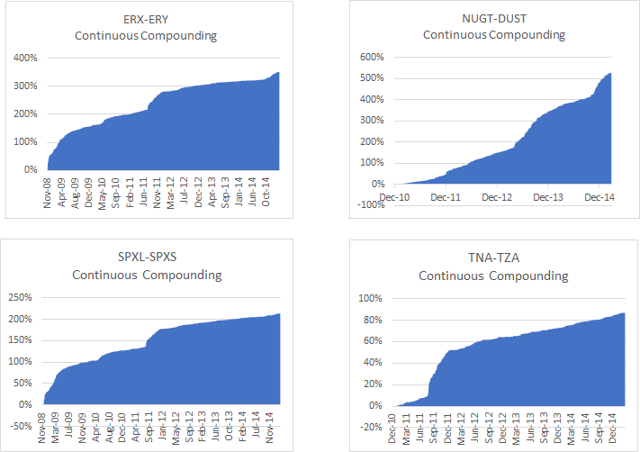
First, let’s look the returns in the ETF portfolios measured using continuous compounding.
Source: Yahoo! Finance

The portfolio returns look very impressive, with CAGRs ranging from around 20% for the short TNA-TZA pair, to over 124% for the short NUGT-DUST pair. Sharpe ratios, too, appear abnormally large, ranging from 4.5 for the ERX-ERY short pair to 8.4 for NUGT-DUST.

Now let’s look at the performance of the same portfolios measured using daily compounding.
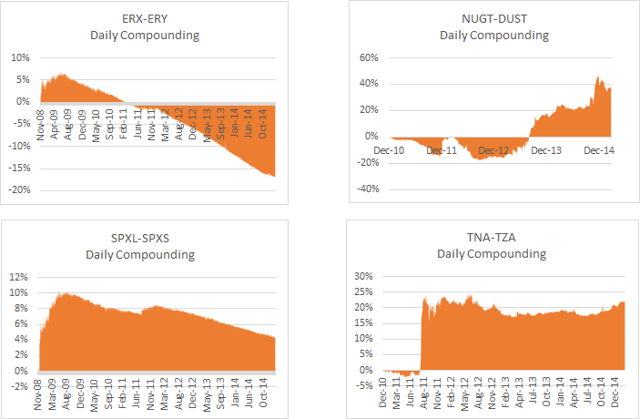
Source: Yahoo! Finance

It’s an altogether different picture. None of the portfolios demonstrate an attract performance record and indeed in two cases the CAGR is negative.

What’s going on?

Stock Loan Costs

Before providing the explanation, let’s just get one important detail out of the way. Since you are shorting both legs of the ETF pairs, you will be faced with paying stock borrow costs. Borrow costs for leveraged ETFs can be substantial and depending on market conditions amount to as much as 10% per annum, or more.

In computing the portfolio returns in both the continuous and daily compounding scenarios I have deducted annual stock borrow costs based on recent average quotes from Interactive Brokers, as follows:

  • ERX-ERY: 14%
  • NUGT-DUST: 16%
  • SXPL-SPXS: 8%
  • TNA-TZA: 8%

It’s All About Compounding and Rebalancing

The implicit assumption in the computation of the daily compounded returns shown above is that you are rebalancing the portfolios each day. That is to say, it is assumed that at the end of each day you buy or sell sufficient quantities of shares of each ETF to maintain an equal $ value in both legs.

In the case of continuously compounded returns the assumption you are making is that you maintain an equal $ value in both legs of the portfolio at every instant. Clearly that is impossible.

Ok, so if the results from low frequency rebalancing are poor, while the results for instantaneous rebalancing are excellent, it is surely just a question of rebalancing the portfolio as frequently as is practically possible. While we may not be able to achieve the ideal result from continuous rebalancing, the results we can achieve in practice will reflect how close we can come to that ideal, right?

Unfortunately, not.

Because, while we have accounted for stock borrow costs, what we have ignored in the analysis so far are transaction costs.

Transaction Costs

With daily rebalancing transaction costs are unlikely to be a critical factor – one might execute a single trade towards the end of the trading session. But in the continuous case, it’s a different matter altogether.

Let’s use the SPXL-SPXS pair as an illustration. When the S&P 500 index declines, the value of the SPXL ETF will fall, while the value of the SPXS ETF will rise. In order to maintain the same $ value in both legs you will need to sell more shares in SPXL and buy back some shares in SPXS. If the market trades up, SPXL will increase in value, while the price of SPXS will fall, requiring you to buy back some SPXL shares and sell more SPXS.

In other words, to rebalance the portfolio you will always be trying to sell the ETF that has declined in price, while attempting to buy the inverse ETF that has appreciated. It is often very difficult to execute a sale in a declining stock at the offer price, or buy an advancing stock at the inside bid. To be sure of completing the required rebalancing of the portfolio, you are going to have to buy at the ask price and sell at the bid price, paying the bid-offer spread each time.

Spreads in leveraged ETF products tend to be large, often several pennies. The cumulative effect of repeatedly paying the bid-ask spread, while taking trading losses on shares sold at the low or bought at the high, will be sufficient to overwhelm the return you might otherwise hope to make from the ETF decay.

And that’s assuming the best case scenario that shares are always available to short. Often they may not be: so that, if the market trades down and you need to sell more SPXL, there may be none available and you will be unable to rebalance your portfolio, even if you were willing to pay the additional stock loan costs and bid-ask spread.

A Lose-Lose Proposition

So, in summary: if you rebalance infrequently you will avoid excessive transaction costs; but the $ imbalance that accrues over the course of a trading day will introduce a market bias in the portfolio. That can hurt portfolio returns very badly if you get caught on the wrong side of a major market move. The results from daily rebalancing for the illustrative pairs shown above indicate that this is likely to happen all too often.

On the other hand, if you try to maintain market neutrality in the portfolio by rebalancing at high frequency, the returns you earn from decay will be eaten up by transaction costs and trading losses, as you continuously sell low and buy high, paying the bid-ask spread each time.

Either way, you lose.

Ok, what about if you reverse the polarity of the portfolio, going long both legs? Won’t that avoid the very high stock borrow costs and put you in a better position as regards the transaction costs involved in rebalancing?

Yes, it will. Because, you will be selling when the market trades up and buying when it falls, making it much easier to avoid paying the bid-ask spread. You will also tend to make short term trading profits by selling high and buying low. Unfortunately, you may not be surprised to learn, these advantages are outweighed by the cost of the decay incurred in both legs of the long ETF portfolio.

In other words: you can expect to lose if you are short; and lose if you are long!

An Analogy from Option Theory

To anyone with a little knowledge of basic option theory, what I have been describing should sound like familiar territory.

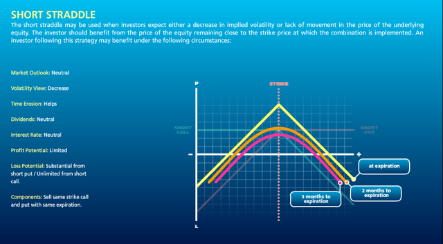
Being short the ETF pair is like being short an option (actually a pair of call and put options, called a straddle). You earn decay, or Theta, for those familiar with the jargon, by earning the premium on the options you have sold; but at the risk of being short Gamma – which measures your exposure to a major market move.
Source: Interactive Brokers

You can hedge out the portfolio’s Gamma exposure by trading the underlying securities – the ETF pair in this case – and when you do that you find yourself always having to sell at the low and buy at the high. If the options are fairly priced, the option decay is enough, but not more, to compensate for the hedging cost involved in continuously trading the underlying.

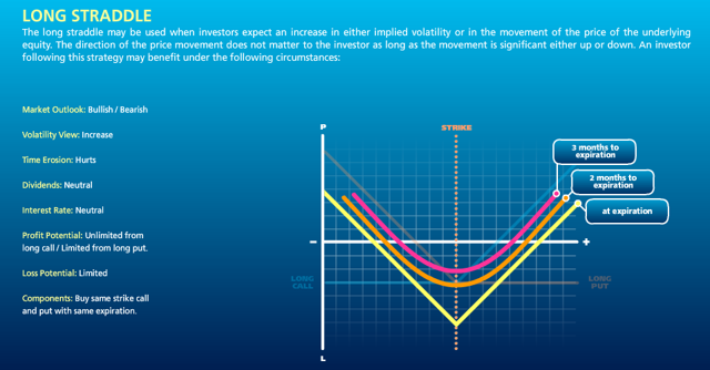
Conversely, being long the ETF pair is like being long a straddle on the underling pair. You now have positive Gamma exposure, so your portfolio will make money from a major market move in either direction. However, the value of the straddle, initially the premium you paid, decays over time at a rate Theta (also known as the “bleed”).
Source: Interactive Brokers

You can offset the bleed by performing what is known as Gamma trading. When the market trades up your portfolio delta becomes positive, i.e. an excess $ value in the long ETF leg, enabling you to rebalance your position by selling excess deltas at the high. Conversely, when the market trades down, your portfolio delta becomes negative and you rebalance by buying the underlying at the current, reduced price. In other words, you sell at the high and buy at the low, typically making money each time. If the straddle is fairly priced, the profits you make from Gamma trading will be sufficient to offset the bleed, but not more.

Typically, the payoff from being short options – being short the ETF pair – will show consistent returns for sustained periods, punctuated by very large losses when the market makes a significant move in either direction.

Conversely, if you are long options – long the ETF pair – you will lose money most of the time due to decay and occasionally make a very large profit.

In an efficient market in which securities are fairly priced, neither long nor short option strategy can be expected to dominate the other in the long run. In fact, transaction costs will tend to produce an adverse outcome in either case! As with most things in life, the house is the player most likely to win.

Developing a Leveraged ETF Strategy that Works

Investors shouldn’t be surprised that it is hard to make money simply by shorting leveraged ETF pairs, just as it is hard to make money by selling options, without risking blowing up your account.

And yet, many traders do trade options and often manage to make substantial profits. In some cases traders are simply selling options, hoping to earn substantial option premiums without taking too great a hit when the market explodes. They may get away with it for many years, before blowing up. Indeed, that has been the case since 2009. But who would want to be an option seller here, with the market at an all-time high? It’s simply far too risky.

The best option traders make money by trading both the long and the short side. Sure, they might lean in one direction or the other, depending on their overall market view and the opportunities they find. But they are always hedged, to some degree. In essence what many option traders seek to do is what is known as relative value trading – selling options they regard as expensive, while hedging with options they see as being underpriced. Put another way, relative value traders try to buy cheap Gamma and sell expensive Theta.

This is how one can thread the needle in leveraged ETF strategies. You can’t hope to make money simply by being long or short all the time – you need to create a long/short ETF portfolio in which the decay in the ETFs you are short is greater than in the ETFs you are long. Such a strategy is, necessarily, tactical: your portfolio holdings and net exposure will likely change from long to short, or vice versa, as market conditions shift. There will be times when you will use leverage to increase your market exposure and occasions when you want to reduce it, even to the point of exiting the market altogether.

If that sounds rather complicated, I’m afraid it is. I have been developing and trading arbitrage strategies of this kind since the early 2000s, often using sophisticated option pricing models. In 2012 I began trading a volatility strategy in ETFs, using a variety of volatility ETF products, in combination with equity and volatility index futures.

I have reproduced the results from that strategy below, to give some indication of what is achievable in the ETF space using relative value arbitrage techniques.
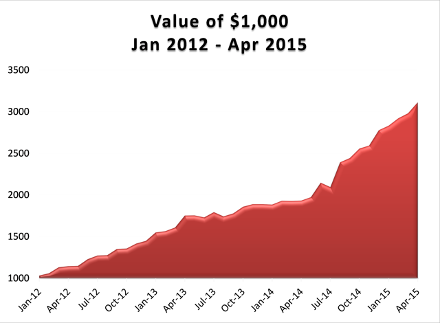
Source: Systematic Strategies, LLC

Source: Systematic Strategies LLC

Conclusion

There are no free lunches in the market. The apparent high performance of strategies that engage systematically in shorting leveraged ETFs is an illusion, based on a failure to quantify the full costs of portfolio rebalancing.

The payoff from a short leveraged ETF pair strategy will be comparable to that of a short straddle position, with positive decay (Theta) and negative Gamma (exposure to market moves). Such a strategy will produce positive returns most of the time, punctuated by very large drawdowns.

The short Gamma exposure can be mitigated by continuously rebalancing the portfolio to maintain dollar neutrality. However, this will entail repeatedly buying ETFs as they trade up and selling them as they decline in value. The transaction costs and trading losses involved in continually buying high and selling low will eat up most, if not all, of the value of the decay in the ETF legs.

A better approach to trading ETFs is relative value arbitrage, in which ETFs with high decay rates are sold and hedged by purchases of ETFs with relatively low rates of decay.

An example given of how this approach has been applied successfully in volatility ETFs since 2012.
Is Your Trading Strategy Still Working?

The Challenge of Validating Strategy Performance

One of the challenges faced by investment strategists is to assess whether a strategy is continuing to perform as it should.  This applies whether it is a new strategy that has been backtested and is now being traded in production, or a strategy that has been live for a while.
All strategies have a limited lifespan.  Markets change, and a trading strategy that can’t accommodate that change will get out of sync with the market and start to lose money. Unless you have a way to identify when a strategy is no longer in sync with the market, months of profitable trading can be undone very quickly.

The issue is particularly important for quantitative strategies.  Firstly, quantitative strategies are susceptible to the risk of over-fitting.  Secondly, unlike a strategy based on fundamental factors, it may be difficult for the analyst to verify that the drivers of strategy profitability remain intact.

Savvy investors are well aware of the risk of quantitative strategies breaking down and are likely to require reassurance that a period of underperformance is a purely temporary phenomenon.

It might be tempting to believe that you will simply stop trading when the strategy stops working.  But given the stochastic nature of investment returns, how do you distinguish a losing streak from a system breakdown?

SSALGOTRADING AD

Stochastic Process Control

One approach to the problem derives from the field of Monte Carlo simulation and stochastic process control.  Here we random draw samples from the distribution of strategy returns and use these to construct a prediction envelope to forecast the range of future returns.  If the equity curve of the strategy over the forecast period  falls outside of the envelope, it would raise serious concerns that the strategy may have broken down.  In those circumstances you would almost certainly want to trade the strategy in smaller size for a while to see if it recovers, or even exit the strategy altogether it it does not.

I will illustrate the procedure for the long/short ETF strategy that I described in an earlier post, making use of Michael Bryant’s excellent Market System Analyzer software.

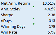
To briefly refresh, the strategy is built using cointegration theory to construct long/short portfolios is a selection of ETFs that provide exposure to US and international equity, currency, real estate and fixed income markets.  The out of sample back-test performance of the strategy is very encouraging:

Fig 2


Fig 1

There was evidently a significant slowdown during 2014, with a reduction in the risk-adjusted returns and win rate for the strategy:

Fig 1

This period might itself have raised questions about the continuing effectiveness of the strategy.  However, we have the benefit of hindsight in seeing that, during the first two months of 2015, performance appeared to be recovering.

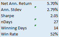
Consequently we put the strategy into production testing at the beginning of March 2015 and we now wish to evaluate whether the strategy is continuing on track.   The results indicate that strategy performance has been somewhat weaker than we might have hoped, although this is compensated for by a significant reduction in strategy volatility, so that the net risk-adjusted returns remain somewhat in line with recent back-test history.

Fig 3

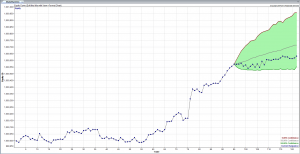
Using the MSA software we sample the most recent back-test returns for the period to the end of Feb 2015, and create a 95% prediction envelope for the returns since the beginning of March, as follows:

Fig 2

As we surmised, during the production period the strategy has slightly underperformed the projected median of the forecast range, but overall the equity curve still falls within the prediction envelope.  As this stage we would tentatively conclude that the strategy is continuing to perform within expected tolerance.

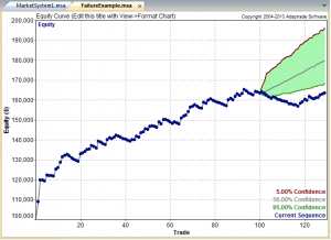
Had we seen a pattern like the one shown in the chart below, our conclusion would have been very different.

Fig 4

As shown in the illustration, the equity curve lies below the lower boundary of the prediction envelope, suggesting that the strategy has failed. In statistical terms, the trades in the validation segment appear not to belong to the same statistical distribution of trades that preceded the validation segment.

This strategy failure can also be explained as follows: The equity curve prior to the validation segment displays relatively little volatility. The drawdowns are modest, and the equity curve follows a fairly straight trajectory. As a result, the prediction envelope is fairly narrow, and the drawdown at the start of the validation segment is so large that the equity curve is unable to rise back above the lower boundary of the envelope. If the history prior to the validation period had been more volatile, it’s possible that the envelope would have been large enough to encompass the equity curve in the validation period.

 CONCLUSION

Systematic trading has the advantage of reducing emotion from trading because the trading system tells you when to buy or sell, eliminating the difficult decision of when to “pull the trigger.” However, when a trading system starts to fail a conflict arises between the need to follow the system without question and the need to stop following the system when it’s no longer working.

Stochastic process control provides a technical, objective method to determine when a trading strategy is no longer working and should be modified or taken offline. The prediction envelope method extrapolates the past trade history using Monte Carlo analysis and compares the actual equity curve to the range of probable equity curves based on the extrapolation.

Next we will look at nonparametric distributions tests  as an alternative method for assessing strategy performance.

The Lazarus Effect

A perennial favorite with investors, presumably because they are easy to understand and implement, are trades based on a regularly occurring pattern, preferably one that is seasonal in nature.  A well-known example is the Christmas effect, wherein equities generally make their highest risk-adjusted returns during the month of December (and equity indices make the greater proportion of their annual gains in the period from November to January).

As we approach the Easter holiday I thought I might join in the fun with a trade of my own.  There being not much new under the sun, I can assume that there is some ancient trader’s almanac that documents the effect I am about to describe.  If so, I apologize in advance if this is duplicative.

The Pattern of Returns in the S&P 500 Index Around Easter

I want to look at the pattern of pre- and post- Easter returns in the S&P 500 index using weekly data from 1950  (readers can of course substitute the index, ETF or other tradable security in a similar analysis).

The first question is whether there are significant differences (economic and statistical) in index returns in the weeks before and after Easter, compared to a regular week.

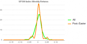
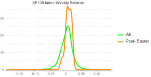
Fig 1

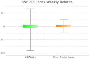
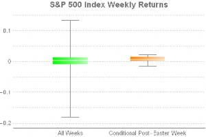
It is perhaps not immediately apparent from the smooth histogram plot above, but a whisker plot gives a clearer indication of the disparity in the distributions of returns in the post-Easter week vs. regular weeks.

Fig 2

It is evident that chief distinction is not in the means of the distributions, but in their variances.

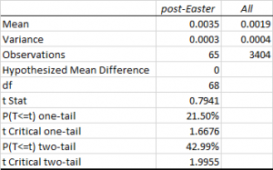
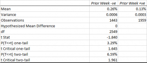
A t-test (with unequal variances) confirms that the difference in average returns in the index in the post-Easter week vs. normal weeks is not statistically significant.

Fig 3 It appears that there is nothing special about Index returns in the post-Easter period.

SSALGOTRADING AD

The Lazarus Effect

Hold on – not so fast.  Suppose we look at conditional returns: that is to say, we consider returns in the post-Easter week for holiday periods in which the index sold off in the  week prior to Easter.

There are 26 such periods in the 65 years since 1950 and when we compare the conditional distribution of index returns for these periods against the unconditional distribution of weekly returns we appear to find significant differences in the distributions.  Not only is the variance of the conditional returns much tighter, the mean is clearly higher than the unconditional weekly returns.

Fig 6


Fig 5


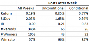
The comparison is perhaps best summarized in the following table.  Here we can see that the average conditional return is more than twice that of the unconditional return in the post-Easter week and almost 4x as large as the average weekly return in the index.  The standard deviation in conditional returns for the post-Easter week is less than half that of the unconditional weekly return, producing and information ratio that is almost 10x larger.  Furthermore, of the 26 periods in which the index return in the week prior to Easter was negative, 22 (85%) produced a positive return in the week after Easter (compared to a win rate of only 57% for unconditional weekly returns.

Fig 4

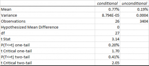
A t-test of conditional vs. unconditional weekly returns confirms that the 58bp difference in conditional vs unconditional (all weeks) average returns is statistically significant at the 0.2% level.

Fig 7

Our initial conclusion, therefore, is that there appears to be a statistically significant pattern in the conditional returns in the S&P 500 index around the post-Easter week. Specifically, the returns in the post-Easter week tend to be much higher than average for  periods in which the pre-Easter weekly returns were negative.

More simply, the S&P 500 index tends to rebound strongly in the week after Easter – a kind of “Lazarus” effect.

 Lazarus – Or Not?

Hold on – not so fast.   What’s so special about Easter?  Yes, I realize it’s topical.  But isn’t this so-called Lazarus effect just a manifestation of the usual mean-reversion in equity index returns?  There is a tendency for weekly returns in the S&P 500 index to “correct” in the week after a downturn.  Maybe the Lazarus effect isn’t specific to Easter.

To examine this hypothesis we need to compare two sets of conditional weekly returns in the S&P 500 index:

A:  Weeks in which the prior week’s return was negative

B:  the subset of A which contains only post-Easter weeks

 If the difference in average returns for sets A and B is not statistically significant, we would conclude that the so-called Lazarus effect is just a manifestation of the commonplace mean reversion in weekly returns.  Only if the average return for the B data set is significant higher than that for set A would we be able to conclude that, in addition to normal mean reversion at weekly frequency, there is an incremental effect specific to the Easter period – the Lazarus effect.

Let’s begin by establishing that there is a statistically significant mean reversion effect in weekly returns in the S&P 500 Index.  Generally, we expect a fall in the index to be followed by a rise (and perhaps vice versa). So we need to  compare the returns in the index for weeks in which the preceding week’s return was positive, vs weeks in which the preceding week’s return was negative.  The t-test below shows the outcome.

Fig 9

The average return in weeks following a downturn is approximately double that during weeks following a rally and the effect is statistically significant at the 3% level.

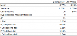
Given that result, is there any incremental “Lazarus” effect around Easter?  We test that hypothesis by comparing the average returns during the 26 post-Easter weeks which were preceded by a downturn in the index against the average return for all 1,444 weeks which followed a decline in the index.

The t-test shown in the table below confirms that conditional returns in post-Easter weeks are approximately 3x larger on average than returns for all weeks that followed a decline in the index.

Fig 8

Lazarus, it appears, is alive and well.

Happy holidays, all.

Combining Momentum and Mean Reversion Strategies

The Fama-French World

For many years now the “gold standard” in factor models has been the 1996 Fama-French 3-factor model: Fig 1
Here r is the portfolio’s expected rate of return, Rf is the risk-free return rate, and Km is the return of the market portfolio. The “three factor” β is analogous to the classical β but not equal to it, since there are now two additional factors to do some of the work. SMB stands for “Small [market capitalization] Minus Big” and HML for “High [book-to-market ratio] Minus Low”; they measure the historic excess returns of small caps over big caps and of value stocks over growth stocks. These factors are calculated with combinations of portfolios composed by ranked stocks (BtM ranking, Cap ranking) and available historical market data. The Fama–French three-factor model explains over 90% of the diversified portfolios in-sample returns, compared with the average 70% given by the standard CAPM model.

The 3-factor model can also capture the reversal of long-term returns documented by DeBondt and Thaler (1985), who noted that extreme price movements over long formation periods were followed by movements in the opposite direction. (Alpha Architect has several interesting posts on the subject, including this one).

Fama and French say the 3-factor model can account for this. Long-term losers tend to have positive HML slopes and higher future average returns. Conversely, long-term winners tend to be strong stocks that have negative slopes on HML and low future returns. Fama and French argue that DeBondt and Thaler are just loading on the HML factor.

SSALGOTRADING AD

Enter Momentum

While many anomalies disappear under  tests, shorter term momentum effects (formation periods ~1 year) appear robust. Carhart (1997) constructs his 4-factor model by using FF 3-factor model plus an additional momentum factor. He shows that his 4-factor model with MOM substantially improves the average pricing errors of the CAPM and the 3-factor model. After his work, the standard factors of asset pricing model are now commonly recognized as Value, Size and Momentum.

 Combining Momentum and Mean Reversion

In a recent post, Alpha Architect looks as some possibilities for combining momentum and mean reversion strategies.  They examine all firms above the NYSE 40th percentile for market-cap (currently around $1.8 billion) to avoid weird empirical effects associated with micro/small cap stocks. The portfolios are formed at a monthly frequency with the following 2 variables:

  1. Momentum = Total return over the past twelve months (ignoring the last month)
  2. Value = EBIT/(Total Enterprise Value)

They form the simple Value and Momentum portfolios as follows:

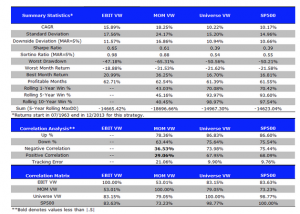
  1. EBIT VW = Highest decile of firms ranked on Value (EBIT/TEV). Portfolio is value-weighted.
  2. MOM VW = Highest decile of firms ranked on Momentum. Portfolio is value-weighted.
  3. Universe VW = Value-weight returns to the universe of firms.
  4. SP500 = S&P 500 Total return

The results show that the top decile of Value and Momentum outperformed the index over the past 50 years.  The Momentum strategy has stronger returns than value, on average, but much higher volatility and drawdowns. On a risk-adjusted basis they perform similarly. Fig 2   The researchers then form the following four portfolios:

  1. EBIT VW = Highest decile of firms ranked on Value (EBIT/TEV). Portfolio is value-weighted.
  2. MOM VW = Highest decile of firms ranked on Momentum. Portfolio is value-weighted.
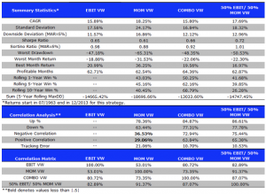
  3. COMBO VW = Rank firms independently on both Value and Momentum.  Add the two rankings together. Select the highest decile of firms ranked on the combined rankings. Portfolio is value-weighted.
  4. 50% EBIT/ 50% MOM VW = Each month, invest 50% in the EBIT VW portfolio, and 50% in the MOM VW portfolio. Portfolio is value-weighted.

With the following results:

Fig 3 The main takeaways are:

  • The combined ranked portfolio outperforms the index over the same time period.
  • However, the combination portfolio performs worse than a 50% allocation to Value and a 50% allocation to Momentum.

A More Sophisticated Model

Yangru Wu of Rutgers has been doing interesting work in this area over the last 15 years, or more. His 2005 paper (with Ronald Balvers), Momentum and mean reversion across national equity markets, considers joint momentum and mean-reversion effects and allows for complex interactions between them. Their model is of the form Fig 4 where the excess return for country i (relative to the global equity portfolio) is represented by a combination of mean-reversion and autoregressive (momentum) terms. Balvers and Wu  find that combination momentum-contrarian strategies, used to select from among 18 developed equity markets at a monthly frequency, outperform both pure momentum and pure mean-reversion strategies. The results continue to hold after corrections for factor sensitivities and transaction costs. The researchers confirm that momentum and mean reversion occur in the same assets. So in establishing the strength and duration of the momentum and mean reversion effects it becomes important to control for each factor’s effect on the other. The momentum and mean reversion effects exhibit a strong negative correlation of 35%. Accordingly, controlling for momentum accelerates the mean reversion process, and controlling for mean reversion may extend the momentum effect.

 Momentum, Mean Reversion and Volatility

The presence of  strong momentum and mean reversion in volatility processes provides a rationale for the kind of volatility strategy that we trade at Systematic Strategies.  One  sophisticated model is the Range Based EGARCH model of  Alizadeh, Brandt, and Diebold (2002) .  The model posits a two-factor volatility process in which a short term, transient volatility process mean-reverts to a stochastic long term mean process, which may exhibit momentum, or long memory effects  (details here).

In our volatility strategy we model mean reversion and momentum effects derived from the level of short and long term volatility-of-volatility, as well as the forward volatility curve. These are applied to volatility ETFs, including levered ETF products, where convexity effects are also important.  Mean reversion is a well understood phenomenon in volatility, as, too, is the yield roll in volatility futures (which also impacts ETF products like VXX and XIV).

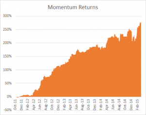
Momentum effects are perhaps less well researched in this context, but our research shows them to be extremely important.  By way of illustration, in the chart below I have isolated the (gross) returns generated by one of the momentum factors in our model.

Fig 6


Developing Long/Short ETF Strategies

Recently I have been working on the problem of how to construct large portfolios of cointegrated securities.  My focus has been on ETFs rather that stocks, although in principle the methodology applies equally well to either, of course.

My preference for ETFs is due primarily to the fact that  it is easier to achieve a wide diversification in the portfolio with a more limited number of securities: trading just a handful of ETFs one can easily gain exposure, not only to the US equity market, but also international equity markets, currencies, real estate, metals and commodities. Survivorship bias, shorting restrictions  and security-specific risk are also less of an issue with ETFs than with stocks (although these problems are not too difficult to handle).

On the downside, with few exceptions ETFs tend to have much shorter histories than equities or commodities.  One also has to pay close attention to the issue of liquidity. That said, I managed to assemble a universe of 85 ETF products with histories from 2006 that have sufficient liquidity collectively to easily absorb an investment of several hundreds of  millions of dollars, at minimum.

The Cardinality Problem

The basic methodology for constructing a long/short portfolio using cointegration is covered in an earlier post.   But problems arise when trying to extend the universe of underlying securities.  There are two challenges that need to be overcome.

Magic Cube.112

The first issue is that, other than the simple regression approach, more advanced techniques such as the Johansen test are unable to handle data sets comprising more than about a dozen securities. The second issue is that the number of possible combinations of cointegrated securities quickly becomes unmanageable as the size of the universe grows.  In this case, even taking a subset of just six securities from the ETF universe gives rise to a total of over 437 million possible combinations (85! / (79! * 6!).  An exhaustive test of all the possible combinations of a larger portfolio of, say, 20 ETFs, would entail examining around 1.4E+19 possibilities.

Given the scale of the computational problem, how to proceed? One approach to addressing the cardinality issue is sparse canonical correlation analysis, as described in Identifying Small Mean Reverting Portfolios,  d’Aspremont (2008). The essence of the idea is something like this. Suppose you find that, in a smaller, computable universe consisting of just two securities, a portfolio comprising, say, SPY and QQQ was  found to be cointegrated.  Then, when extending consideration to portfolios of three securities, instead of examining every possible combination, you might instead restrict your search to only those portfolios which contain SPY and QQQ. Having fixed the first two selections, you are left with only 83 possible combinations of three securities to consider.  This process is repeated as you move from portfolios comprising 3 securities to 4, 5, 6, … etc.

Other approaches to the cardinality problem are  possible.  In their 2014 paper Sparse, mean reverting portfolio selection using simulated annealing,  the Hungarian researchers Norbert Fogarasi and Janos Levendovszky consider a new optimization approach based on simulated annealing.  I have developed my own, hybrid approach to portfolio construction that makes use of similar analytical methodologies. Does it work?

A Cointegrated Long/Short ETF Basket

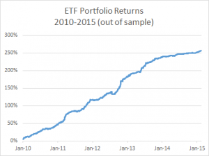
Below are summarized the out-of-sample results for a portfolio comprising 21 cointegrated ETFs over the period from 2010 to 2015.  The basket has broad exposure (long and short) to US and international equities, real estate, currencies and interest rates, as well as exposure in banking, oil and gas and other  specific sectors.

The portfolio was constructed using daily data from 2006 – 2009, and cointegration vectors were re-computed annually using data up to the end of the prior year.  I followed my usual practice of using daily data comprising “closing” prices around 12pm, i.e. in the middle of the trading session, in preference to prices at the 4pm market close.  Although liquidity at that time is often lower than at the close, volatility also tends to be muted and one has a period of perhaps as much at two hours to try to achieve the arrival price. I find this to be a more reliable assumption that the usual alternative.

Fig 2   Fig 1 The risk-adjusted performance of the strategy is consistently outstanding throughout the out-of-sample period from 2010.  After a slowdown in 2014, strategy performance in the first quarter of 2015 has again accelerated to the level achieved in earlier years (i.e. with a Sharpe ratio above 4).

Another useful test procedure is to compare the strategy performance with that of a portfolio constructed using standard mean-variance optimization (using the same ETF universe, of course).  The test indicates that a portfolio constructed using the traditional Markowitz approach produces a similar annual return, but with 2.5x the annual volatility (i.e. a Sharpe ratio of only 1.6).  What is impressive about this result is that the comparison one is making is between the out-of-sample performance of the strategy vs. the in-sample performance of a portfolio constructed using all of the available data.

Having demonstrated the validity of the methodology,  at least to my own satisfaction, the next step is to deploy the strategy and test it in a live environment.  This is now under way, using execution algos that are designed to minimize the implementation shortfall (i.e to minimize any difference between the theoretical and live performance of the strategy).  So far the implementation appears to be working very well.

Once a track record has been built and audited, the really hard work begins:  raising investment capital!