MATH-TWS: Connecting Wolfram Mathematica to IB TWS

Mathematica can now connect to Interactive Brokers Trader Workstation

At long last, it’s here!

MATH-TWS is a new Mathematica package that connects Wolfram Mathematica to the Interactive Brokers TWS platform via the C++ API. It enables the user to retrieve information from TWS on accounts, portfolios and positions, as well as historical and real-time market data. MATH-TWS also enables the user to place and amend orders and obtain execution confirmations from Mathematica.

In the following sections we will illustrate the functionality of the MATH-TWS package using the full functional form and show the abbreviated equivalent form in comments.


Conclusions:  Connecting Mathematica to IB TWS

I have wanted a way to connect Wolfram Mathematica to Interactive Brokers’ Trader Workstation for the longest time.  Now that it is finally available with MATH-TWS  I am excited by the possibilities for Mathematica users.

The first release of MATH-TWS will be available within a couple of weeks. Anyone interested in licensing a copy should email algorithmicexecution@gmail.com with MATH-TWS in the subject line.


Algorithmic Trading

MOVING FROM RESEARCH TO TRADING

I have written recently about the comparative advantages of different programming languages in the context of research and trading (see here).  My sense of it is that there is no single “ideal” programming language – the best strategy is to pick an appropriate tool for the job and there are usually several reasonable choices one could make.

If you are engaged in econometrics research, you might choose a package like RATS, Eviews, Gauss, or Prof. James Davidson’s excellent and inexpensive TSM, which I have used for many years and can recommend highly. For a latency-sensitive high frequency trading application, you will probably want to use something like C++, or possibly a 3rd party algo system like Apama or Tethys. But for algorithmic trading systems of intermediate frequency the choice appears almost unlimited.

Matlab AlgoThe problem with retail trading tools like TradeStation, Multicharts, or Amibroker, is that they are designed primarily for single-asset strategies.  That may be ok for futures trading,where more often than not the focus is on a single underlying, but in equities the opposite is true. Using one of these products to develop and implement a pairs trading strategy is a stretch.   As for portfolio analytics – forget it.

This is where more general, high level languages like R, Matlab or Mathematica come in:  their greater power and flexibility is handling large, multivariate data sets makes it much more straightforward to develop portfolio strategies. And they can often bridge the gap between R&D and implementation quite easily:  code that was used in the research stage can often be quickly re-tooled to work in a production version of the system.  As for production systems, there is now a significant cottage industry of traders who use Matlab in algo trading.  R has a similar following (see here).

In addition to parallelizing the code (for use with the Parallel Computing Toolbox) to speed up the research phase, you might also want to implement a hybrid system by re-coding the slower routines in C++, to create a mex file (for details see here). Matlab’s Profiler is a useful tool for identifying code bottlenecks.  In a recent piece of research in which I was evaluating over 30,000,000 cointegrated portfolios, I discovered to my surprise that the main code bottleneck was the multiple calls to Matlab’s std function, a problem easily fixed with a few lines of C++ code.  The resulting hybrid program executed at more than twice the speed – important when your run time might be several hours, or even days.

HOOKING UP THE EXECUTION PLATFORM

The main challenge for developers using generic tools like Mathematica, Matlab or R is the implementation stage of the project. Providing connectivity to brokerage/execution platforms never seemed high on the list of priorities for Wolfram or Mathworks and things are similarly hit or miss with R.

Belatedly, Mathematica now offers a link to Bloomberg via its Finance Platform.  Matlab, meanwhile, offers a Trading Toolbox, which supposedly offers connectivity , not only to Bloomberg, but also Interactive Brokers and Trading Technologies, amongst other platforms.  Unfortunately, the toolbox interface to IB appears to rely on outdated 1990s ActiveX technology, which is flakey at best.  In tests, I was unable to make progress past the ‘not connected’ error message.

At that point I turned to Yair Altman’s  IB-Matlab product.  Happily, this uses IB’s Java api, which is a great deal more robust than the ActiveX platform.  It’s been some time since I last used IB-Matlab and was pleased to see that Yair has been very busy over the intervening period, building the capabilities of the system and providing very comprehensive documentation for it.  With Yair’s help, it took me no time at all to get up and running and within a day or two the system was executing orders flawlessly in IB’s TWS.  The relatively few snags I ran into were almost all due to IB’s extremely terse error messaging, which often gives almost no clue as to what the issue might be.  Fortunately, Yair is very generous with his time in providing support to his users and his responses to me questions were fast and detailed.

EXECUTION ALGOS

With intermediate  systems trading at frequencies of, say, 5-minutes to daily, one has a choice to make as regards execution.  Given that the strategy is not very latency sensitive, it is certainly conceivable to develop one’s own execution algos in Matlab.  However, platforms like TWS are equipped with native algos, not only from IB, but also other providers like Credit Suisse and JefAD Algofries.

Actually, I have found several of IB’s own algos such as Scaletrader and Accumulate/Distribute to be very effective. Certainly IB seems very proud of them – IB CEO Thomas Peterffy has patented at least one of them. Accumulate/Distribute, for instance, is quite sophisticated, allowing the user to randomize and slice the size and interval between individual orders, use passive or aggressive order types, and pause execution on a news alert, or when the price falls below a moving average, or outside a specified range.

There is much to be said for using algos native to the execution platform rather than reinventing the wheel, providing the cost is reasonable. So, while it is perfectly feasible to build execution algos in Matlab, it typically isn’t necessary – in most cases standard algos will suffice.

There are exceptions, of course.  IB doesn’t offer the  kind of basket-trading capabilities REDIthat are available in advanced algo platforms like Tethys or RediPlus.  In those systems, for example, you can set the level of long/short imbalance in the portfolio that you are willing to tolerate and the algo will speed up or slow down execution of trades in individual components of the basket to maintain the dollar imbalance within that tolerance.  You can also manage the sector risk dynamically during execution.

Those kind of advanced capabilities don’t come cheap and you wont find them at IB, or any other retail platform. If you need that kind of functionality, for example, because you are trading a long/short equity portfolio within a universe of 200-300 names, your best option is probably to switch to a different execution platform.  Otherwise you will need to code a custom algo in your language of choice.

For many quantitative strategies, (at least the low frequency ones) IB’s standard algos are often good enough.  The Accumulate/Distribute algo, for instance, will show a visual representation of the progress of the execution of individuals legs of a pairs trade, and it is easy enough to identify a potential imbalance and adjust the algo parameters in real time. If you are only trading pairs, or small portfolios of cointegrated securities, it probably isn’t worthwhile to develop the sophisticated logic that would be required to handle the adjustment of the execution of individual legs of a trade in a fully automated way.  A large portfolio would be a different matter, however.

MATLAB EXAMPLE

I thought it might be instructive to take a look at how you might implement the execution of a strategy in Matlab, using IB algos. In the Matlab code fragment below, the (2 x nTickers) array tradeActions contains, in the first row, the action we wish to take (1 = BUY, -1 = SELL, -2 = SELL SHORT) and in the second row the (absolute value of) the number of shares we wish to trade for tickers i =1:nTickers. We break each order up into hundred lots and odd lots, routing the former via IB’s Accumulate/Distribute algo and the latter as passive REL orders (note that A/D  will typically randomize the timing of each sub-order, while REL orders are posted directly into the market). The Matlab function AccumulateDistribute implements the most important features of IB’s A/D algo, including random size and time slicing of the order.  Orders are submitted as passive REL orders with zero offset (so they will sit on the current bid or ask) – obviously you would typically want to consider allowing some non-zero offset for less liquid securities.  It is not hard to envisage how one might further enhance the algo to monitor the progress of the execution and speed up or slow down certain orders accordingly.

MatlabA couple of IB api “gotchas” to be aware of:

(i) IB requires unique and monotonically increasing orderIds for each order. One way to do this, suggested by Yair, is to use orderId = round((now-735000)*3e5);  This fails when you are submitting a number of orders sequentially at high speed (say in a for loop), where the time increments are sub-second, so you need to pass the orderID back and force a minimal increment, as I have in the code below.

(ii) It is very important to specify the primary exchange of each security:  securities with identical tickers can be found trading on different exchanges.  Failing to specify the primary exchange in such a case will result in IB rejecting the order with a typically cryptic api message.

Continue reading “Algorithmic Trading”

Cointegration Breakdown

The Low Power of Cointegration Tests

One of the perennial difficulties in developing statistical arbitrage strategies is the lack of reliable methods of estimating a stationary portfolio comprising two or more securities. In a prior post (below) I discussed at some length one of the primary reasons for this, i.e. the lower power of cointegration tests. In this post I want to explore the issue in more depth, looking at the standard Johansen test Procedure to estimate cointegrating vectors.

Johansen Test for Cointegration

Start with some weekly data for an ETF triplet analyzed in Ernie Chan’s book:

After downloading the weekly close prices for the three ETFs we divide the data into 14 years of in-sample data and 1 year out of sample:

We next apply the Johansen test, using code kindly provided by Amanda Gerrish:

We find evidence of up to three cointegrating vectors at the 95% confidence level:


Let’s take a look at the vector coefficients (laid out in rows, in Amanda’s function):

In-Sample vs. Out-of-Sample testing

We now calculate the in-sample and out-of-sample portfolio values using the first cointegrating vector:

The portfolio does indeed appear to be stationary, in-sample, and this is confirmed by the unit root test, which rejects the null hypothesis of a unit root:

Unfortunately (and this is typically the case) the same is not true for the out of sample period:

More Data Doesn’t Help

The problem with the nonstationarity of the out-of-sample estimated portfolio values is not mitigated by adding more in-sample data points and re-estimating the cointegrating vector(s):

We continue to add more in-sample data points, reducing the size of the out-of-sample dataset correspondingly. But none of the tests for any of the out-of-sample datasets is able to reject the null hypothesis of a unit root in the portfolio price process:


The Challenge of Cointegration Testing in Real Time

In our toy problem we know the out-of-sample prices of the constituent ETFs, and can therefore test the stationarity of the portfolio process out of sample. In a real world application, that discovery could only be made in real time, when the unknown, future ETFs prices are formed. In that scenario, all the researcher has to go on are the results of in-sample cointegration analysis, which demonstrate that the first cointegrating vector consistently yields a portfolio price process that is very likely stationary in sample (with high probability).

The researcher might understandably be persuaded, wrongly, that the same is likely to hold true in future. Only when the assumed cointegration relationship falls apart in real time will the researcher then discover that it’s not true, incurring significant losses in the process, assuming the research has been translated into some kind of trading strategy.

A great many analysts have been down exactly this path, learning this important lesson the hard way. Nor do additional “safety checks” such as, for example, also requiring high levels of correlation between the constituent processes add much value. They might offer the researcher comfort that a “belt and braces” approach is more likely to succeed, but in my experience it is not the case: the problem of non-stationarity in the out of sample price process persists.

Conclusion:  Why Cointegration Breaks Down

We have seen how a portfolio of ETFs consistently estimated to be cointegrated in-sample, turns out to be non-stationary when tested out-of-sample.  This goes to the issue of the low power of cointegration test, and their inability to estimate cointegrating vectors with sufficient accuracy.  Analysts relying on standard tests such as the Johansen procedure to design their statistical arbitrage strategies are likely to be disappointed by the regularity with which their strategies break down in live trading.


Successful Statistical Arbitrage


I tend not to get involved in Q&A with readers of my blog, or with investors.  I am at a point in my life where I spend my time mostly doing what I want to do, rather than what other people would like me to do.  And since I enjoy doing research and trading, I try to maximize the amount of time I spend on those activities.

As a business strategy, I wouldn’t necessarily recommend this approach.  It’s just something I evolved while learning to play chess: since I had no-one to teach me, I had to learn everything for myself and this involved studying for many, many hours alone.

By contrast, several of the best money managers are also excellent communicators – take Roy Niederhoffer, or Ernie Chan, for example. Having regular, informed communication with your investors is, as smarter managers have realized, a means of building trust and investor loyalty – important factors that come into play during periods when your strategy is underperforming. Not only that, but since communication is two-way, an analyst/manager can learn much from his exchanges with his clients.  Knowing how others perceive you – and your competitors – for example, is very useful information.  So, too, is information about your competitors’ research ideas, investment strategies and fund performance, which can often be gleaned from discussions with investors.  There are plenty of reasons to prefer a policy of regular, open communication.

As a case in point, I was surprised to learn from  comments on another research blog that readers drew the conclusion from my previous posts that pursuing the cointegration or Kalman Filter approach to statistical arbitrage was a waste of time.  Apparently, my remark to the effect that researchers often failed to pay attention to the net PnL per share in evaluating stat. arb. trading strategies was taken by some to mean that any apparent profitability would always be subsumed within the bid-offer spread.  That was not my intention.  What I intended to convey was that in some instances, this would be the case  – some, but not all.

To illustrate the point, below are the out-of-sample results from a research study applying the Kalman Filter approach for four equity pairs using 5-minute data.  For competitive reasons I am unable to identify the specific stocks in each pair, which result from an exhaustive analysis of over 30,000 pairs, but I can say that they are liquid large-cap equities traded in large volume on the US exchanges.  The performance numbers are net of transaction costs and are based on the assumption of a 5-minute delay in execution: meaning, a trading signal received at time t is assumed to be executed at time t+5 minutes.  This allows sufficient time to leg into each trade passively, in most cases avoiding the bid-offer spread.  The net PnL per share is above 1.5c per share for each pair.

Fig 0 While the performance of none of the pairs is spectacular, a combined portfolio has quite attractive characteristics, which include 81% winning months since Jan 2012, a CAGR of over 27% and Information Ratio of 2.29, measured on monthly returns (2.74 based on daily returns).

Fig 2

Fig 3

Finally, I am currently implementing trading of a number of stock portfolios based on static cointegration relationships that have out-of-sample information ratios of between 3 and 4, using daily data.


A Comparison of Programming Languages

Towards the end of last year I wrote a post (see here) about the advent of modern programming languages, including the JIT compiled Julia and visual programming language ADL from Trading Technologies.  My conclusion (based on a not very scientific sample) was that we appear to be at the tipping point, where the speed of newer, high level languages  languages is approaching that of the fastest compiled languages like C/C++.

Now comes a formal academic study of the topic in A Comparison of Programming Languages in Economics, Aruoba and Fernandez-Villaverde, 2014.  Using the neoclassical growth model, the authors conduct a benchmark test in C++11, Fortran 2008, Java, Julia, Python, Matlab, Mathematica, and R, implementing the same algorithm, value function
iteration with grid search, in each of the languages. They report the execution times of the codes in a Mac and in a Windows computer and briefly comment on the strengths and weaknesses of each language.

The conclusions from the study mirror my own thoughts on the subject very closely. The authors find that:

  1. C++ and Fortran are still considerably faster than any other alternative, although one needs to be careful with the choice of compiler.
  2. C++ compilers have advanced enough that, contrary to the situation in the 1990s and some folk wisdom, C++ code runs slightly faster (5-7 percent) than Fortran code.
  3. Julia delivers outstanding performance. Execution speed is only between 2.64 and 2.70 times slower than the execution speed of the best C++ compiler.
  4. Baseline Python was slow. Using the Pypy implementation, it runs around 44 times slower than in C++. Using the default CPython interpreter, the code runs between 155 and 269 times slower than in C++.
  5. Matlab is between 9 to 11 times slower than the best C++ executable.
  6. R runs between 475 to 491 times slower than C++. If the code is compiled, the code is between 243 to 282 times slower.
  7. Hybrid programming and special approaches can deliver considerable speed ups. For example, when combined with Mex files, Matlab is only 1.24 to 1.64 times slower than C++ and when combined with Rcpp, R is between 3.66 and 5.41 times slower. Similar numbers hold for Numba (a just-in-time compiler for Python that uses decorators) and Cython (a static compiler for writing C extensions for Python) in the Python ecosystem.
  8. Mathematica is only about three times slower than C++, but only after a considerable rewriting of the code to take advantage of the peculiarities of the language. The baseline version of the algorithm in Mathematica is considerably slower.

C++ still represents the benchmark for speed, but not by much.  It is barely faster than the old stalwart, Fortran, and only 1.5 – 3 times faster than up-and-coming rivals amongst the higher level languages (especially when you allow for hybrid programming to speed up the slowest algorithms).c++

So, as regards developing financial models and trading systems, my questions are (as before):

  • Why would anyone prefer Python, given that there is a much faster, free alternative in Julia, which is just as easy a language to program in?
  • What justification is there for preferring R to Matlab, other than cost?
  • Why does anyone bother with Java?  If speed is the critical issue, there are faster alternatives.  If you like the relative simplicity of the syntax, Julia is cleaner, simpler and just as fast in execution.

When you reach a point where a high level language like Matlab is only around 1.5x – 2x slower than C++, you really have to question whether the latter is an appropriate choice.  Yes, of course, in mission-critical applications where you need access to the hardware layer for speed purposes, C++ is the way to go.  But for so many applications, that just isn’t the case.

What matters, far, far more, are the months of costly and laborious programming effort that is often required to reproduce basic functionality that is already embedded in higher level languages like Matlab or Mathematica.  Not only that, but the end result of a C++ /Java development effort is likely to be notoriously inflexible by comparison.  That’s a huge drawback.  Rarely, if ever, does a piece of research translate flawlessly into production – it requires one to iterate towards a final solution, often making significant changes to the design of the system in the light of practical experience.

If I had to guess, based on my experience, I would say that 80% or more of development tasks in quantitative research and trading would produce a superior result if preference was given to using a higher level language for the initial development.  When the system is sufficiently stable to put into production, you simply create a hybrid application by recoding any mission-critical components for which speed is an issue in C++.

Finally, where does that leave my beloved Mathematica?  To be fair, while you don’t have the joys of strong typing to contend with, Mathematica’s syntax is just as demanding and uncompromising as C++ – a missed comma or incorrectly placed bracket is just as critical.  But, the point is, while in C++ the syntactical rigor is just annoying, in Mathematica it’s worth putting up with because the productivity is so much greater.  A competent programmer can produce, in a single line of Mathematica code, a program that would require hundreds, if not thousands of lines of C++ code to accomplish.  Sure, he might get the syntax wrong at first:  but it’s only a single line of code and the interactive gui interface makes debugging very simple.


mathematica fn

That said, while Mathematica can be very tedious to use for procedural programming, it excels in three areas:

1.  Symbolic programming. Anything involving mathematical symbols and equations – Mathematica is #1

2.  User interface.  In Mathematica, it is trivial to build a  sophisticated, dynamic gui in no time at all, again, often in 1-2 lines of code

3.  Functional programming. Anything that can be thought of as a function, Mathematica handles extremely well.  We are not talking about finding a square root here:  I mean extremely complex functions that, again, might take hundreds of lines of code in another language.

It is also worth pointing out that Mathematica comes supplied with functionality that Matlab provides only through numerous, costly add-on packages.

CONCLUSION
Before I allow a development team to start mindlessly coding up a system in Java or C++, I want to hear their reasons why they aren’t going to do it 10x faster in another, higher level language.  “We always use C++/Java for production” is not a reason.  Specifically, which parts of the system require the additional 1.5x speed-up, and why can’t they be coded as dlls (Matlab mex functions)?

Finally, on a cost-benefit basis, ask yourself how much  you might benefit if the months and tens (or hundreds) of thousands of dollars wasted on developing in C++ were instead spent on researching and developing new trading ideas.


Quant Strategies in 2018

Quant Strategies – Performance Summary Sept. 2018

The end of Q3 seems like an appropriate time for an across-the-piste review of how systematic strategies are performing in 2018.  I’m using the dozen or more strategies running on the Systematic Algotrading Platform as the basis for the performance review, although results will obviously vary according to the specifics of the strategy.  All of the strategies are traded live and performance results are net of subscription fees, as well as slippage and brokerage commissions.

Volatility Strategies

Those waiting for the hammer to fall on option premium collecting strategies will have been disappointed with the way things have turned out so far in 2018.  Yes, February saw a long-awaited and rather spectacular explosion in volatility which completely destroyed several major volatility funds, including the VelocityShares Daily Inverse VIX Short-Term ETN (XIV) as well as Chicago-based hedged fund LJM Partners (“our goal is to preserve as much capital as possible”), that got caught on the wrong side of the popular VIX carry trade.  But the lack of follow-through has given many volatility strategies time to recover. Indeed, some are positively thriving now that elevated levels in the VIX have finally lifted option premiums from the bargain basement levels they were languishing at prior to February’s carnage.  The Option Trader strategy is a stand-out in this regard:  not only did the strategy produce exceptional returns during the February melt-down (+27.1%), the strategy has continued to outperform as the year has progressed and YTD returns now total a little over 69%.  Nor is the strategy itself exceptionally volatility: the Sharpe ratio has remained consistently above 2 over several years.

Hedged Volatility Trading

Investors’ chief concern with strategies that rely on collecting option premiums is that eventually they may blow up.  For those looking for a more nuanced approach to managing tail risk the Hedged Volatility strategy may be the way to go.  Like many strategies in the volatility space the strategy looks to generate alpha by trading VIX ETF products;  but unlike the great majority of competitor offerings, this strategy also uses ETF options to hedge tail risk exposure.  While hedging costs certainly acts as a performance drag, the results over the last few years have been compelling:  a CAGR of 52% with a Sharpe Ratio close to 2.

F/X Strategies

One of the common concerns for investors is how to diversify their investment portfolios, especially since the great majority of assets (and strategies) tend to exhibit significant positive correlation to equity indices these days. One of the characteristics we most appreciate about F/X strategies in general and the F/X Momentum strategy in particular is that its correlation to the equity markets over the last several years has been negligible.    Other attractive features of the strategy include the exceptionally high win rate – over 90% – and the profit factor of 5.4, which makes life very comfortable for investors.  After a moderate performance in 2017, the strategy has rebounded this year and is up 56% YTD, with a CAGR of 64.5% and Sharpe Ratio of 1.89.

Equity Long/Short

Thanks to the Fed’s accommodative stance, equity markets have been generally benign over the last decade to the benefit of most equity long-only and long-short strategies, including our equity long/short Turtle Trader strategy , which is up 31% YTD.  This follows a spectacular 2017 (+66%) , and is in line with the 5-year CAGR of 39%.   Notably, the correlation with the benchmark S&P500 Index is relatively low (0.16), while the Sharpe Ratio is a respectable 1.47.

Equity ETFs – Market Timing/Swing Trading

One alternative to the traditional equity long/short products is the Tech Momentum strategy.  This is a swing trading strategy that exploits short term momentum signals to trade the ProShares UltraPro QQQ (TQQQ) and ProShares UltraPro Short QQQ (SQQQ) leveraged ETFs.  The strategy is enjoying a banner year, up 57% YTD, with a four-year CAGR of 47.7% and Sharpe Ratio of 1.77.  A standout feature of this equity strategy is its almost zero correlation with the S&P 500 Index.  It is worth noting that this strategy also performed very well during the market decline in Feb, recording a gain of over 11% for the month.

Futures Strategies

It’s a little early to assess the performance of the various futures strategies in the Systematic Strategies portfolio, which were launched on the platform only a few months ago (despite being traded live for far longer).    For what it is worth, both of the S&P 500 E-Mini strategies, the Daytrader and the Swing Trader, are now firmly in positive territory for 2018.   Obviously we are keeping a watchful eye to see if the performance going forward remains in line with past results, but our experience of trading these strategies gives us cause for optimism.

Conclusion:  Quant Strategies in 2018

There appear to be ample opportunities for investors in the quant sector across a wide range of asset classes.  For investors with equity market exposure, we particularly like strategies with low market correlation that offer significant diversification benefits, such as the F/X Momentum and F/X Momentum strategies.  For those investors seeking the highest risk adjusted return, option selling strategies like the Option Trader strategy are the best choice, while for more cautious investors concerned about tail risk the Hedged Volatility strategy offers the security of downside protection.  Finally, there are several new strategies in equities and futures coming down the pike, several of which are already showing considerable promise.  We will review the performance of these newer strategies at the end of the year.

Go here for more information about the Systematic Algotrading Platform.

ETF Pairs Trading with the Kalman Filter

I was asked by a reader if I could illustrate the application of the Kalman Filter technique described in my previous post with an example. Let’s take the ETF pair AGG IEF, using daily data from Jan 2006 to Feb 2015 to estimate the model.  As you can see from the chart in Fig. 1, the pair have been highly correlated over the last several years.

Fig 1Fig 1.  AGG and IEF Daily Prices 2006-2015

We now estimate the beta-relationship between the ETF pair with the Kalman Filter, using the Matlab code given below, and plot the estimated vs actual prices of the first ETF, AGG in Fig 2.  There are one or two outliers that you might want to take a look at, but mostly the fit looks very good. Fig 2

 Fig 2 – Actual vs Fitted Prices of AGG

Now lets take a look at Kalman Filter estimates of beta.  As you can see in Fig 3, it wanders around a lot!  Very difficult to handle using some kind of static beta estimate. Fig 3

Fig 3 – Kalman Filter Beta Estimates

  Finally, we compute the raw and standardized alphas, being the differences between the observed and fitted prices , i.e. Alpha(t) = AGG(t) – b(t)* IEF(t) and kfAlpha(t) = (Alpha(t) – mean(Alpha(t)) / std(Alpha(t)   I have plotted the kfAlpha estimates over the last year in Fig 4.   Fig 4

Fig 4 – Standardized Alpha Estimates

  The last step is to decide how to trade this relationship.  You might, for example, trade the portfolio in proportion to the standardized deviation (i.e. the  size of kfAlpha(t)).  Alternatively, you might set a threshold level, say +/- 1 Sd, and trade the portfolio when  kfAlpha(t) exceeds this the threshold.   In the Matlab code below I use the particle swarm method  to maximize the likelihood.  I have found this to be more reliable than other methods.

Continue reading “ETF Pairs Trading with the Kalman Filter”

Statistical Arbitrage Using the Kalman Filter

One of the challenges with the cointegration approach to statistical arbitrage which I discussed in my previous post, is that cointegration relationships are seldom static: they change quite frequently and often break down completely.  Back in 2009 I began experimenting with a more dynamic approach to pairs trading, based on the Kalman Filter.


In its simplest form, we  model the relationship between a pair of securities in the following way:

beta(t) = beta(t-1) + w     beta(t), the unobserved state variable, that follows a random walk

Y(t) = beta(t)X(t) + v      The observed processes of stock prices Y(t) and X(t)

where:

w ~ N(0,Q) meaning w is gaussian noise with zero mean and variance Q

v ~ N(0,R) meaning v is gaussian noise with variance R

So this is just like the usual pairs relationship Y = beta * X + v, where the typical approach is to estimate beta using least squares regression, or some kind of rolling regression (to try to take account of the fact that beta may change over time).  In this traditional framework, beta is static, or slowly changing.

In the Kalman framework, beta is itself a random process that evolves continuously over time, as a random walk.  Because it is random and contaminated by noise we cannot observe beta directly, but must infer its (changing) value from the observable stock prices X and Y. (Note: in what follows I shall use X and Y to refer to stock prices.  But you could also use log prices, or returns).

Unknown to me at that time,  several other researchers were thinking along the same lines and later published their research.  One such example is Statistical Arbitrage and High-Frequency Data with an Application to Eurostoxx 50 Equities,  Rudy, Dunis, Giorgioni and Laws, 2010.  Another closely related study is  Performance Analysis of Pairs Trading Strategy Utilizing High Frequency Data with an Application to KOSPI 100 Equities, Kim, 2011.  Both research studies follow a very similar path, rejecting beta estimation using rolling regression or exponential smoothing in favor of the Kalman approach and applying a Ornstein-Uhlenbeck model to estimate the half-life of mean reversion of the pairs portfolios.  The studies report very high out-of-sample information ratios that in some cases exceed 3.

I have already made the point that such unusually high performance is typically the result of ignoring the fact that the net PnL per share may lie within the region of the average bid-offer spread, making implementation highly problematic.  In this post I want to dwell on another critical issue that is particular to the Kalman approach: the signal:noise ratio, Q/R, which expresses the ratio of the variance of the beta process to that of the price process.  (Curiously, both papers make the same mistake of labelling Q and R as standard deviations. In fact, they are variances).

Beta, being a random process, obviously contains some noise:  but the hope is that it is less noisy than the price process.  The idea is that the relationship between two stocks is more stable – less volatile – than the stock processes themselves.  On its face, that assumption appears reasonable, from an empirical standpoint.  The question is:  how stable is the beta process, relative to the price process? If the variance in the beta process is  low relative to the price process,  we can determine beta quite accurately over time and so obtain accurate estimates of the true price Y(t), based on X(t).  Then, if we observe a big enough departure in the quoted price Y(t) from the true price at time t, we have a potential trade.

In other words, we are interested in:

alpha(t) = Y(t) – Y*(t) = Y(t) – beta(t) X(t)

where Y(t) and X(t) are the observed stock prices and beta(t) is the estimated value of beta at time t.

As usual, we would standardize the alpha using an estimate of the alpha standard deviation, which is sqrt(R).  (Alternatively, you can estimate the standard deviation of the alpha directly, using a lookback period based on the alpha half-life).

If the standardized alpha is large enough, the model suggests that the price Y(t) is quoted significantly in excess of the true value.  Hence we would short stock Y and buy stock X.  (In this context, where X and Y represent raw prices, you would hold an equal and opposite number of shares in Y and X.  If X and Y represented returns, you would hold equal and opposite market value in each stock).

The success of such a strategy depends critically on the quality of our estimates of alpha, which in turn rest on the accuracy of our estimates of beta. This depends on the noisiness of the beta process, i.e. its variance, Q.  If the beta process is very noisy, i.e. if Q is large, our estimates of alpha are going to be too noisy to be useful as the basis for a reversion strategy.

So, the key question I want to address in this post is: in order for the Kalman approach to be effective in modeling a pairs relationship, what would be an acceptable range for the beta process variance Q ?  (It is often said that what matters in the Kalman framework is not the variance Q, per se, but rather the signal:noise ratio Q/R.  It turns out that this is not strictly true, as we shall see).

To get a handle on the problem, I have taken the following approach:

(i) Simulate a stock process X(t) as a geometric brownian motion process with specified drift and volatility (I used 0%,  5% and 10% for the annual drift, and 10%,  30% and 60% for the corresponding annual volatility).

(ii) simulate a beta(t) process as a random walk with variance Q in the range from 1E-10 to 1E-1.

(iii) Generate the true price process Y(t) = beta(t)* X(t)

(iv) Simulate an observed price process Yobs(t), by adding random noise with variance R to Y(t), with R in the range 1E-6 to 1.0

(v) Calculate the true, known alpha(t) = Y(t) – Yobs(t)

(vi) Fit the Kalman Filter model to the simulated processes and estimate beta(t)  and Yest(t). Hence produce estimates kfalpha(t)  = Yobs(t) – Yest(t) and compare these with the known, true alpha(t).

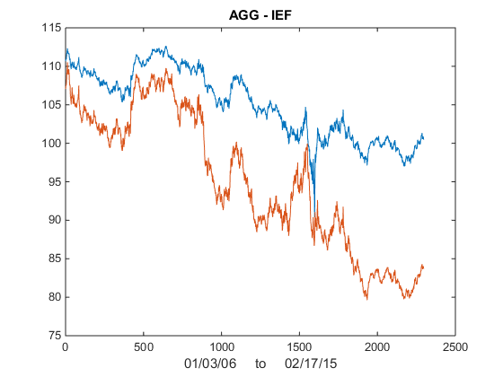
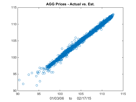
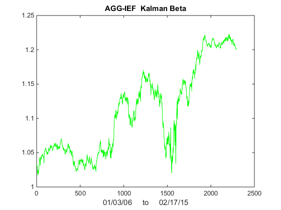
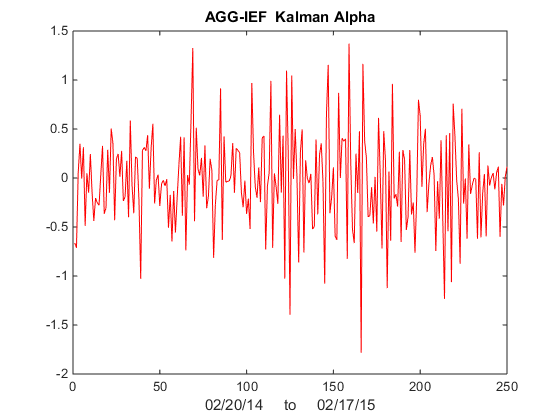
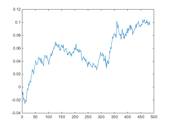
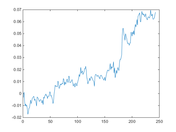
The charts in Fig. 1 below illustrate the procedure for a stock process X(t) with annual drift of 10%, annual volatility 40%, beta process variance Q of 8.65E-9 and price process variance R of 5.62E-2 (Q/R ratio of 1.54E-7).

Fig 1

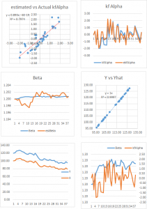
Fig. 1 True and Estimated Beta and Alpha Using the Kalman Filter

As you can see, the Kalman Filter does  a very good job of updating its beta estimate to track the underlying, true beta (which, in this experiment, is known). As the noise ratio Q/R is small, the Kalman Filter estimates of the process alpha, kfalpha(t), correspond closely to the true alpha(t), which again are known to us in this experimental setting.  You can examine the relationship between the true alpha(t) and the Kalman Filter estimates kfalpha(t) is the chart in the upmost left quadrant of the figure.  The correlation between the two is around 89%.  With a level of accuracy this good for our alpha estimates, the pair of simulated stocks would make an ideal candidate for a pairs trading strategy.

Of course, the outcome is highly dependent on the values we assume for Q and R (and also to some degree on the assumptions made about the drift and volatility of the price process X(t)).

The next stage of the analysis is therefore to generate a large number of simulated price and beta observations and examine the impact of different levels of Q and R, the variances of the beta and price process.  The results are summarized in the table in Fig 2 below.

Fig 2

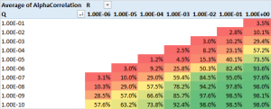
 Fig 2. Correlation between true alpha(t) and kfalpha(t) for values of Q and R

As anticipated, the correlation between the true alpha(t) and the estimates produced by the Kalman Filter is very high when the signal:noise ratio is small, i.e. of the order of 1E-6, or less.  Average correlations begin to tail off very quickly when Q/R exceeds this level, falling to as low as 30% when the noise ratio exceeds 1E-3.  With a Q/R ratio of 1E-2 or higher, the alpha estimates become too noisy to be useful.

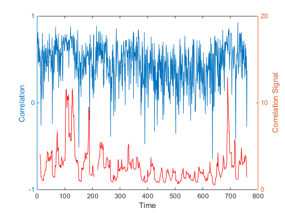
I find it rather fortuitous, even implausible, that in their study Rudy, et al, feel able to assume a noise ratio of 3E-7 for all of the stock pairs in their study, which just happens to be in the sweet spot for alpha estimation.  From my own research, a much larger value in the region of 1E-3 to 1E-5 is  more typical. Furthermore, the noise ratio varies significantly from pair to pair, and over time.  Indeed, I would go so far as to recommend applying a noise ratio filter to the strategy, meaning that trading signals are ignored when the noise ratio exceeds some specified level.

The take-away is this:  the Kalman Filter approach can be applied very successfully in developing statistical arbitrage strategies, but only for processes where the noise ratio is not too large.  One suggestion is to use a filter rule to supress trade signals generated at times when the noise ratio is too large, and/or to increase allocations to pairs in which the noise ratio is relatively low.


Developing Statistical Arbitrage Strategies Using Cointegration

In his latest book (Algorithmic Trading: Winning Strategies and their Rationale, Wiley, 2013) Ernie Chan does an excellent job of setting out the procedures for developing statistical arbitrage strategies using cointegration.  In such mean-reverting strategies, long positions are taken in under-performing stocks and short positions in stocks that have recently outperformed.

I will leave a detailed description of the procedure to Ernie (see pp 47 – 60), which in essence involves:

(i) estimating a cointegrating relationship between two or more stocks, using the Johansen procedure

(ii) computing the half-life of mean reversion of the cointegrated process, based on an Ornstein-Uhlenbeck  representation, using this as a basis for deciding the amount of recent historical data to be used for estimation in (iii)

(iii) Taking a position proportionate to the Z-score of the market value of the cointegrated portfolio (subtracting the recent mean and dividing by the recent standard deviation, where “recent” is defined with reference to the half-life of mean reversion)

Countless researchers have followed this well worn track, many of them reporting excellent results.  In this post I would like to discuss a few of many considerations  in the procedure and variations in its implementation.  We will follow Ernie’s example, using daily data for the EWF-EWG-ITG triplet of ETFs from April 2006 – April 2012. The analysis runs as follows (I am using an adapted version of the Matlab code provided with Ernie’s book):

Johansen test We reject the null hypothesis of fewer then three cointegrating relationships at the 95% level. The eigenvalues and eigenvectors are as follows:

Eigenvalues The eignevectors are sorted by the size of their eigenvalues, so we pick the first of them, which is expected to have the shortest half-life of mean reversion, and create a portfolio based on the eigenvector weights (-1.046, 0.76, 0.2233).  From there, it requires a simple linear regression to estimate the half-life of mean reversion:

Halflife From which we estimate the half-life of mean reversion to be 23 days.  This estimate gets used during the final, stage 3, of the process, when we choose a look-back period for estimating the running mean and standard deviation of the cointegrated portfolio.  The position in each stock (numUnits) is sized according to the standardized deviation from the mean (i.e. the greater the deviation the larger the allocation). Apply Ci The results appear very promising, with an annual APR of 12.6% and Sharpe ratio of 1.4:   Returns EWA-EWC-IGE

Ernie is at pains to point out that, in this and other examples in the book, he pays no attention to transaction costs, nor to the out-of-sample performance of the strategies he evaluates, which is fair enough.

The great majority of the academic studies that examine the cointegration approach to statistical arbitrage for a variety of investment universes do take account of transaction costs.  For the most part such studies report very impressive returns and Sharpe ratios that frequently exceed 3.  Furthermore, unlike Ernie’s example which is entirely in-sample, these studies typically report consistent out-of-sample performance results also.

But the single, most common failing of such studies is that they fail to consider the per share performance of the strategy.  If the net P&L per share is less than the average bid-offer spread of the securities in the investment portfolio, the theoretical performance of the strategy is unlikely to survive the transition to implementation.  It is not at all hard to achieve a theoretical Sharpe ratio of 3 or higher, if you are prepared to ignore the fact that the net P&L per share is lower than the average bid-offer spread.  In practice, however, any such profits are likely to be whittled away to zero in trading frictions – the costs incurred in entering, adjusting and exiting positions across multiple symbols in the portfolio.

Put another way, you would want to see a P&L per share of at least 1c, after transaction costs, before contemplating implementation of the strategy.  In the case of the EWA-EWC-IGC portfolio the P&L per share is around 3.5 cents.  Even after allowing, say, commissions of 0.5 cents per share and a bid-offer spread of 1c per share on both entry and exit, there remains a profit of around 2 cents per share – more than enough to meet this threshold test.

Let’s address the second concern regarding out-of-sample testing.   We’ll introduce a parameter to allow us to select the number of in-sample days, re-estimate the model parameters using only the in-sample data, and test the performance out of sample.  With a in-sample size of 1,000 days, for instance, we find that we can no longer reject the null hypothesis of fewer than 3 cointegrating relationships and the weights for the best linear portfolio differ significantly from those estimated using the entire data set.

Johansen 2

Repeating the regression analysis using the eigenvector weights of the maximum eigenvalue vector (-1.4308, 0.6558, 0.5806), we now estimate the half-life to be only 14 days.  The out-of-sample APR of the strategy over the remaining 500 days drops to around 5.15%, with a considerably less impressive Sharpe ratio of only 1.09.

osPerfOut-of-sample cumulative returns

One way to improve the strategy performance is to relax the assumption of strict proportionality between the portfolio holdings and the standardized deviation in the market value of the cointegrated portfolio.  Instead, we now require  the standardized deviation of the portfolio market value to exceed some chosen threshold level before we open a position (and we close any open positions when the deviation falls below the threshold).  If we choose a threshold level of 1, (i.e. we require the market value of the portfolio to deviate 1 standard deviation from its mean before opening a position), the out-of-sample performance improves considerably:

osPerf 2

The out-of-sample APR is now over 7%, with a Sharpe ratio of 1.45.

The strict proportionality requirement, while logical,  is rather unusual:  in practice, it is much more common to apply a threshold, as I have done here.  This addresses the need to ensure an adequate P&L per share, which will typically increase with higher thresholds.  A countervailing concern, however, is that as the threshold is increased the number of trades will decline, making the results less reliable statistically.  Balancing the two considerations, a threshold of around 1-2 standard deviations is a popular and sensible choice.

Of course, introducing thresholds opens up a new set of possibilities:  just because you decide to enter based on a 2x SD trigger level doesn’t mean that you have to exit a position at the same level.  You might consider the outcome of entering at 2x SD, while exiting at 1x SD, 0x SD, or even -2x SD.  The possible nuances are endless.

Unfortunately, the inconsistency in the estimates of the cointegrating relationships over different data samples is very common.  In fact, from my own research, it is often the case that cointegrating relationships break down entirely out-of-sample, just as do correlations.  A recent study by Matthew Clegg of over 860,000 pairs confirms this finding (On the Persistence of Cointegration in Pais Trading, 2014) that cointegration is not a persistent property.

I shall examine one approach to  addressing the shortcomings  of the cointegration methodology  in a future post.


Matlab code (adapted from Ernie Chan’s book):

Continue reading “Developing Statistical Arbitrage Strategies Using Cointegration”

The Correlation Signal

The use of correlations is widespread in investment management theory and practice, from the construction of portfolios to the design of hedge trades to statistical arbitrage strategies.

A common difficulty encountered in all of these applications is the variation in correlation: assets that at one time appear to be suitably uncorrelated for hedging purposes, may become much more highly correlated at other times, such as periods of market stress. Conversely, stocks that appear suitable for pairs trading due to the high correlation in their prices or returns, may de-couple at a later time, causing significant losses.

The instability in the level of correlation is further aggravated by the empirical finding that the volatility in correlation is itself time-dependent:  at times the correlations between assets may appear to fluctuate smoothly within a tight range; at other times we might see several fluctuations in the sign of the correlation  coefficient over the course of a few days.

One tool I have found useful in this context is a concept I refer to as the correlation signal, defined at the average correlation divided by the standard deviation of the correlation coefficient.  The chart below illustrates a typical pattern for a pair of Oil and Gas industry stocks.  The blue line is the average daily correlation between the stocks, measured at 5-minute intervals.  The red line is the correlation signal – the average daily correlation divided by the standard deviation in the intra-day correlation.  The stochastic nature of both the correlation coefficient and the correlation signal is quite evident.  Note that the correlation signal, unlike the coefficient, is not constrained within the limits of +/- 1.  At times when the variation in correlation is low the signal an easily exceed those limits by as much as an order of magnitude.

CorrSig Plot

In later posts I will illustrate the usefulness of the correlation signal in portfolio construction and statistical arbitrage.  For now, let me just say that it is a measure of the strength of the correlation as a signal, relative to the noise of random variation in the correlation process.   It can be used to identify situations in which a relationship – whether a positive or negative correlation – appears to be stable or unstable, and therefore viable as a basis for inference, or not.