Correlation Cointegration

In a previous post I looked at ways of modeling the relationship between the CBOE VIX Index and the Year 1 and Year 2 CBOE Correlation Indices:

http://jonathankinlay.com/2017/08/modeling-volatility-correlation/

The question was put to me whether the VIX and correlation indices might be cointegrated.

Let’s begin by looking at the pattern of correlation between the three indices:

If you recall from my previous post, we were able to fit a linear regression model with the Year 1 and Year 2 Correlation Indices that accounts for around 50% in the variation in the VIX index. While the model certainly has its shortcomings, as explained in the post, it will serve the purpose of demonstrating that the three series are cointegrated. The standard Dickey-Fuller test rejects the null hypothesis of a unit root in the residuals of the linear model, confirming that the three series are cointegrated, order 1.

Vector Autoregression

We can attempt to take the modeling a little further by fitting a VAR model. We begin by splitting the data into an in-sample period from Jan 2007 to Dec 2015 and an out-of-sample test period from Jan 2016 to Aug 2017. We then fit a vector autoregression model to the in-sample data:

When we examine how the model performs on the out-of-sample data, we find that it fails to pick up on much of the variation in the series – the forecasts are fairly flat and provide quite poor predictions of the trends in the three series over the period from 2016-2017:

Conclusion

The VIX and Correlation Indices are not only highly correlated, but also cointegrated, in the sense that a linear combination of the series is stationary.

One can fit a weakly stationary VAR process model to the three series, but the fit is quite poor and forecasts from the model don’t appear to add much value. It is conceivable that a more comprehensive model involving longer lags would improve forecasting performance.

March 24, 2020

Modeling Volatility and Correlation

In a previous blog post I mentioned the VVIX/VIX Ratio, which is measured as the ratio of the CBOE VVIX Index to the VIX Index. The former measures the volatility of the VIX, or the volatility of volatility.

http://jonathankinlay.com/2017/07/market-stress-test-signals-danger-ahead/

A follow-up article in ZeroHedge shortly afterwards pointed out that the VVIX/VIX ratio had reached record highs, prompting Goldman Sachs analyst Ian Wright to comment that this could signal the ending of the current low-volatility regime:

A linkedIn reader pointed out that individual stock volatility was currently quite high and when selling index volatility one is effectively selling stock correlations, which had now reached historically low levels. I concurred:

What’s driving the low vol regime is the exceptionally low level of cross-sectional correlations. And, as correlations tighten, index vol will rise. Worse, we are likely to see a feedback loop – higher vol leading to higher correlations, further accelerating the rise in index vol. So there is a second order, Gamma effect going on. We see that is the very high levels of the VVIX index, which shot up to 130 last week. The all-time high in the VVIX prior to Aug 2015 was around 120. The intra-day high in Aug 2015 reached 225. I’m guessing it will get back up there at some point, possibly this year.

As there appears to be some interest in the subject I decided to add a further blog post looking a little further into the relationship between volatility and correlation. To gain some additional insight we are going to make use of the CBOE implied correlation indices. The CBOE web site explains:

Using SPX options prices, together with the prices of options on the 50 largest stocks in the S&P 500 Index, the CBOE S&P 500 Implied Correlation Indexes offers insight into the relative cost of SPX options compared to the price of options on individual stocks that comprise the S&P 500.

CBOE calculates and disseminates two indexes tied to two different maturities, usually one year and two years out. The index values are published every 15 seconds throughout the trading day.

Both are measures of the expected average correlation of price returns of S&P 500 Index components, implied through SPX option prices and prices of single-stock options on the 50 largest components of the SPX.

Dispersion Trading

One application is dispersion trading, which the CBOE site does a good job of summarizing:

The CBOE S&P 500 Implied Correlation Indexes may be used to provide trading signals for a strategy known as volatility dispersion (or correlation) trading. For example, a long volatility dispersion trade is characterized by selling at-the-money index option straddles and purchasing at-the-money straddles in options on index components. One interpretation of this strategy is that when implied correlation is high, index option premiums are rich relative to single-stock options. Therefore, it may be profitable to sell the rich index options and buy the relatively inexpensive equity options.

The VIX Index and the Implied Correlation Indices

Again, the CBOE web site is worth quoting:

The CBOE S&P 500 Implied Correlation Indexes measure changes in the relative premium between index options and single-stock options. A single stock’s volatility level is driven by factors that are different from what drives the volatility of an Index (which is a basket of stocks). The implied volatility of a single-stock option simply reflects the market’s expectation of the future volatility of that stock’s price returns. Similarly, the implied volatility of an index option reflects the market’s expectation of the future volatility of that index’s price returns. However, index volatility is driven by a combination of two factors: the individual volatilities of index components and the correlation of index component price returns.

Let’s dig into this analytically. We first download and plot the daily for the VIX and Correlation Indices from the CBOE web site, from which it is evident that all three series are highly correlated:

An inspection reveals significant correlations between the VIX index and the two implied correlation indices, which are themselves highly correlated. The S&P 500 Index is, of course, negatively correlated with all three indices:

Modeling Volatility-Correlation

The response surface that describes the relationship between the VIX index and the two implied correlation indices is locally very irregular, but the slope of the surface is generally positive, as we would expect, since the level of VIX correlates positively with that of the two correlation indices.

The most straightforward approach is to use a simple linear regression specification to model the VIX level as a function of the two correlation indices. We create a VIX Model Surface object using this specification with the Mathematica Predict function:The linear model does quite a good job of capturing the positive gradient of the response surface, and in fact has a considerable amount of explanatory power, accounting for a little under half the variance in the level of the VIX index:

However, there are limitations. To begin with, the assumption of independence between the explanatory variables, the correlation indices, clearly does not hold. In cases such as this, where explanatory variables are multicolinear, we are unable to draw inferences about the explanatory power of individual regressors, even though the model as a whole may be highly statistically significant, as here.

Secondly, a linear regression model is not going to capture non-linearities in the volatility-correlation relationship that are evident in the surface plot. This is confirmed by a comparison plot, which shows that the regression model underestimates the VIX level for both low and high values of the index:

We can achieve a better outcome using a machine learning algorithm such as nearest neighbor, which is able to account for non-linearities in the response surface:

The comparison plot shows a much closer correspondence between actual and predicted values of the VIX index, even though there is evidence of some remaining heteroscedasticity in the model residuals:

Conclusion

A useful way to think about index volatility is as a two dimensional process, with time-series volatility measured on one dimension and dispersion (cross-sectional volatility, the inverse of correlation) measured on the second. The two factors are correlated and, as we have shown here, interact in a complicated, non-linear way.

The low levels of index volatility we have seen in recent months result, not from low levels of volatility in component stocks, but in the historically low levels of correlation (high levels of dispersion) in the underlying stock returns processes. As correlations begin to revert to historical averages, the impact will be felt in an upsurge in index volatility, compounded by the non-linear interaction between the two factors.

March 17, 2020March 17, 2020

Tactical Mutual Fund Strategies

A recent blog post of mine was posted on Seeking Alpha (see summary below if you missed it).

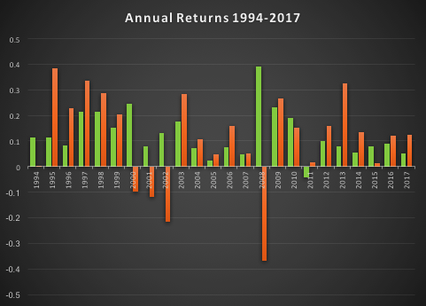
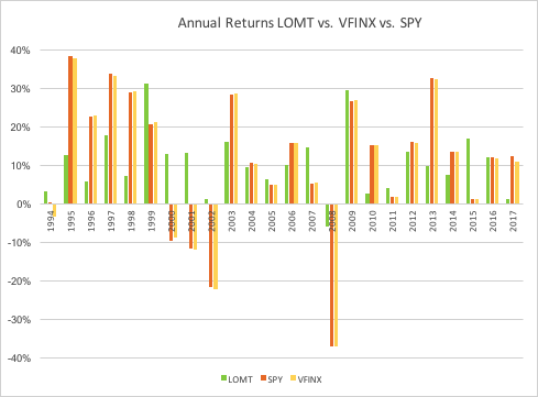
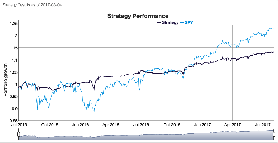
The essence of the idea is simply that one can design long-only, tactical market timing strategies that perform robustly during market downturns, or which may even be positively correlated with volatility. I used the example of a LOMT (“Long-Only Market-Timing”) strategy that switches between the SPY ETF and 91-Day T-Bills, depending on the current outlook for the market as characterized by machine learning algorithms. As I indicated in the article, the LOMT handily outperforms the buy-and-hold strategy over the period from 1994 -2017 by several hundred basis points:

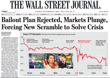
Of particular note is the robustness of the LOMT strategy performance during the market crashes in 2000/01 and 2008, as well as the correction in 2015:

The Pros and Cons of Market Timing (aka “Tactical”) Strategies

One of the popular choices the investor concerned about downsize risk is to use put options (or put spreads) to hedge some of the market exposure. The problem, of course, is that the cost of the hedge acts as a drag on performance, which may be reduced by several hundred basis points annually, depending on market volatility. Trying to decide when to use option insurance and when to maintain full market exposure is just another variation on the market timing problem.

The point of tactical strategies is that, unlike an option hedge, they will continue to produce positive returns – albeit at a lower rate than the market portfolio – during periods when markets are benign, while at the same time offering much superior returns during market declines, or crashes. If the investor is concerned about the lower rate of return he is likely to achieve during normal years, the answer is to make use of leverage.

Market timing strategies like Hull Tactical or the LOMT have higher risk-adjusted rates of return (Sharpe Ratios) than the market portfolio. So the investor can make use of margin money to scale up his investment to about the same level of risk as the market index. In doing so he will expect to earn a much higher rate of return than the market.

This is easy to do with products like LOMT or Hull Tactical, because they make use of marginable securities such as ETFs. As I point out in the sections following, one of the shortcomings of applying the market timing approach to mutual funds, however, is that they are not marginable (not initially, at least), so the possibilities for using leverage are severely restricted.

Market Timing with Mutual Funds

An interesting suggestion from one Seeking Alpha reader was to apply the LOMT approach to the Vanguard 500 Index Investor fund (VFINX), which has a rather longer history than the SPY ETF. Unfortunately, I only have ready access to data from 1994, but nonetheless applied the LOMT model over that time period. This is an interesting challenge, since none of the VFINX data was used in the actual construction of the LOMT model. The fact that the VFINX series is highly correlated with SPY is not the issue – it is typically the case that strategies developed for one asset will fail when applied to a second, correlated asset. So, while it is perhaps hard to argue that the entire VFIX is out-of-sample, the performance of the strategy when applied to that series will serve to confirm (or otherwise) the robustness and general applicability of the algorithm.

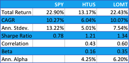
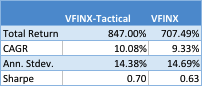
The results turn out as follows:

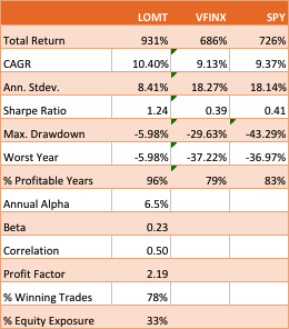
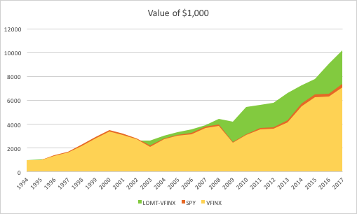
The performance of the LOMT strategy implemented for VFINX handily outperforms the buy-and-hold portfolios in the SPY ETF and VFINX mutual fund, both in terms of return (CAGR) and well as risk, since strategy volatility is less than half that of buy-and-hold. Consequently the risk adjusted return (Sharpe Ratio) is around 3x higher.

That said, the VFINX variation of LOMT is distinctly inferior to the original version implemented in the SPY ETF, for which the trading algorithm was originally designed. Of particular significance in this context is that the SPY version of the LOMT strategy produces substantial gains during the market crash of 2008, whereas the VFINX version of the market timing strategy results in a small loss for that year. More generally, the SPY-LOMT strategy has a higher Sortino Ratio than the mutual fund timing strategy, a further indication of its superior ability to manage downside risk.

Given that the objective is to design long-only strategies that perform well in market downturns, one need not pursue this particular example much further , since it is already clear that the LOMT strategy using SPY is superior in terms of risk and return characteristics to the mutual fund alternative.

Practical Limitations

There are other, practical issues with apply an algorithmic trading strategy a mutual fund product like VFINX. To begin with, the mutual fund prices series contains no open/high/low prices, or volume data, which are often used by trading algorithms. Then there are the execution issues: funds can only be purchased or sold at market prices, whereas many algorithmic trading systems use other order types to enter and exit positions (stop and limit orders being common alternatives). You can’t sell short and there are restrictions on the frequency of trading of mutual funds and penalties for early redemption. And sales loads are often substantial (3% to 5% is not uncommon), so investors have to find a broker that lists the selected funds as no-load for the strategy to make economic sense. Finally, mutual funds are often treated by the broker as ineligible for margin for an initial period (30 days, typically), which prevents the investor from leveraging his investment in the way that he do can quite easily using ETFs.

For these reasons one typically does not expect a trading strategy formulated using a stock or ETF product to transfer easily to another asset class. The fact that the SPY-LOMT strategy appears to work successfully on the VFINX mutual fund product (on paper, at least) is highly unusual and speaks to the robustness of the methodology. But one would be ill-advised to seek to implement the strategy in that way. In almost all cases a better result will be produced by developing a strategy designed for the specific asset (class) one has in mind.

A Tactical Trading Strategy for the VFINX Mutual Fund

A better outcome can possibly be achieved by developing a market timing strategy designed specifically for the VFINX mutual fund. This strategy uses only market orders to enter and exit positions and attempts to address the issue of frequent trading by applying a trading cost to simulate the fees that typically apply in such situations. The results, net of imputed fees, for the period from 1994-2017 are summarized as follows:

Overall, the CAGR of the tactical strategy is around 88 basis points higher, per annum. The risk-adjusted rate of return (Sharpe Ratio) is not as high as for the LOMT-SPY strategy, since the annual volatility is almost double. But, as I have already pointed out, there are unanswered questions about the practicality of implementing the latter for the VFINX, given that it seeks to enter trades using limit orders, which do not exist in the mutual fund world.

The performance of the tactical-VFINX strategy relative to the VFINX fund falls into three distinct periods: under-performance in the period from 1994-2002, about equal performance in the period 2003-2008, and superior relative performance in the period from 2008-2017.

Only the data from 1/19934 to 3/2008 were used in the construction of the model. Data in the period from 3/2008 to 11/2012 were used for testing, while the results for 12/2012 to 8/2017 are entirely out-of-sample. In other words, the great majority of the period of superior performance for the tactical strategy was out-of-sample. The chief reason for the improved performance of the tactical-VFINX strategy is the lower drawdown suffered during the financial crisis of 2008, compared to the benchmark VFINX fund. Using market-timing algorithms, the tactical strategy was able identify the downturn as it occurred and exit the market. This is quite impressive since, as perviously indicated, none of the data from that 2008 financial crisis was used in the construction of the model.

In his Seeking Alpha article “Alpha-Winning Stars of the Bull Market“, Brad Zigler identifies the handful of funds that have outperformed the VFINX benchmark since 2009, generating positive alpha:

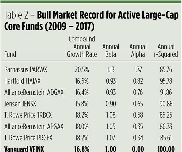
What is notable is that the annual alpha of the tactical-VINFX strategy, at 1.69%, is higher than any of those identified by Zigler as being “exceptional”. Furthermore, the annual R-squared of the tactical strategy is higher than four of the seven funds on Zigler’s All-Star list. Based on Zigler’s performance metrics, the tactical VFINX strategy would be one of the top performing active funds.

But there is another element missing from the assessment. In the analysis so far we have assumed that in periods when the tactical strategy disinvests from the VFINX fund the proceeds are simply held in cash, at zero interest. In practice, of course, we would invest any proceeds in risk-free assets such as Treasury Bills. This would further boost the performance of the strategy, by several tens of basis points per annum, without any increase in volatility. In other words, the annual CAGR and annual Alpha, are likely to be greater than indicated here.

Robustness Testing

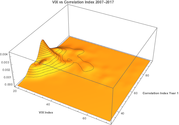
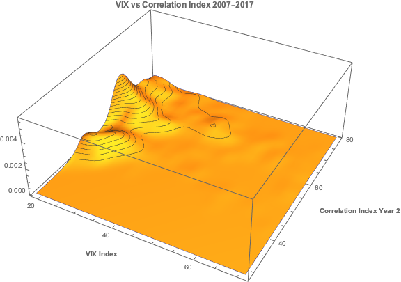
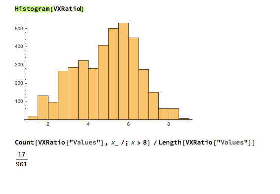
One of the concerns with any backtest – even one with a lengthy out-of-sample period, as here – is that one is evaluating only a single sample path from the price process. Different evolutions could have produced radically different outcomes in the past, or in future. To assess the robustness of the strategy we apply Monte Carlo simulation techniques to generate a large number of different sample paths for the price process and evaluate the performance of the strategy in each scenario.

Three different types of random variation are factored into this assessment:

We allow the observed prices to fluctuate by +/- 30% with a probability of about 1/3 (so, roughly, every three days the fund price will be adjusted up or down by that up to that percentage).
Strategy parameters are permitted to fluctuate by the same amount and with the same probability. This ensures that we haven’t over-optimized the strategy with the selected parameters.
Finally, we randomize the start date of the strategy by up to a year. This reduces the risk of basing the assessment on the outcome from encountering a lucky (or unlucky) period, during which the market may be in a strong trend, for example.

In the chart below we illustrate the outcome from around 1,000 such randomized sample paths, from which it can be seen that the strategy performance is robust and consistent.

Limitations to the Testing Procedure

We have identified one way in which this assessment understates the performance of the tactical-VFINX strategy: by failing to take into account the uplift in returns from investing in interest-bearing Treasury securities, rather than cash, at times when the strategy is out of the market. So it is only reasonable to point out other limitations to the test procedure that may paint a too-optimistic picture.

The key consideration here is the frequency of trading. On average, the tactical-VFINX strategy trades around twice a month, which is more than normally permitted for mutual funds. Certainly, we have factored in additional trading costs to account for early redemptions charges. But the question is whether or not the strategy would be permitted to trade at such frequency, even with the payment of additional fees. If not, then the strategy would have to be re-tooled to work on long average holding periods, no doubt adversely affecting its performance.

Conclusion

The purpose of this analysis was to assess whether, in principle, it is possible to construct a market timing strategy that is capable of outperforming a VFINX fund benchmark. The answer appears to be in the affirmative. However, several practical issues remain to be addressed before such a strategy could be put into production successfully. In general, mutual funds are not ideal vehicles for expressing trading strategies, including tactical market timing strategies. There are latent inefficiencies in mutual fund markets – the restrictions on trading and penalties for early redemption, to name but two – that create difficulties for active approaches to investing in such products – ETFs are much superior in this regard. Nonetheless, this study suggest that, in principle, tactical approaches to mutual fund investing may deliver worthwhile benefits to investors, despite the practical challenges.

March 10, 2020

Capitalizing on the Coming Market Crash

Long-Only Equity Investors

Recently I have been discussing possible areas of collaboration with an RIA contact on LinkedIn, who also happens to be very familiar with the hedge fund world. He outlined the case of a high net worth investor in equities (long only), who wanted to remain invested, but was becoming increasingly concerned about the prospects for a significant market downturn, or even a market crash, similar to those of 2000 or 2008.

I am guessing he is not alone: hardly a day goes by without the publication of yet another article sounding a warning about stretched equity valuations and the dangerously elevated level of the market.

The question put to me was, what could be done to reduce the risk in the investor’s portfolio?

Typically, conservative investors would have simply moved more of their investment portfolio into fixed income securities, but with yields at such low levels this is hardly an attractive option today. Besides, many see the bond market as representing an even more extreme bubble than equities currently.

Hedging Strategies

The problem with traditional hedging mechanisms such as put options, for example, is that they are relatively expensive and can easily reduce annual returns from the overall portfolio by several hundred basis points. Even at current low level of volatility the performance drag is noticeable, since the potential upside in the equity portfolio is also lower than it has been for some time. A further consideration is that many investors are not mandated – or are simply reluctant – to move beyond traditional equity investing into complex ETF products or derivatives.

An equity long/short hedge fund product is one possible solution, but many equity investors are reluctant to consider shorting stocks under any circumstances, even for hedging purposes. And while a short hedge may provide some downside protection it is unlikely to fully safeguard the investor in a crash scenario. Furthermore, the cost of a hedge fund investment is typically greater than for a long-only product, entailing the payment of a performance fee in addition to management fees that are often higher than for standard investment products.

The Ideal Investment Strategy

Given this background, we can say that the ideal investment strategy is one that:

Invests long-only in equities
Is inexpensive to implement (reasonable management fees; no performance fees)
Does not require shorting stocks, or expensive hedging mechanisms such as options
Makes acceptable returns during both bull and bear markets
Is likely to produce positive returns in a market crash scenario

A typical buy-and-hold approach is unlikely to meet only the first three requirements, although an argument could be made that a judicious choice of defensive stocks might enable the investment portfolio to generate returns at an “acceptable” level during a downturn (without being prescriptive as to the precise meaning of that term may be). But no buy-and-hold strategy could ever be expected to prosper during times of severe market stress. A more sophisticated approach is required.

Market Timing

Market timing is regarded as a “holy grail” by some quantitative strategists. The idea, simply, is to increase or reduce risk exposure according to the prospects for the overall market. For a very long time the concept has been dismissed as impossible, by definition, given that markets are mostly efficient. But analysts have persisted in the attempt to develop market timing techniques, motivated by the enormous benefits that a viable market timing strategy would bring. And gradually, over time, evidence has accumulated that the market can be timed successfully and profitably. The rate of progress has accelerated in the last decade by the considerable advances in computing power and the development of machine learning algorithms and application of artificial intelligence to investment finance.

I have written several articles on the subject of market timing that the reader might be interested to review (see below). In this article, however, I want to focus firstly on the work on another investment strategist, Blair Hull.

http://jonathankinlay.com/2014/07/how-to-bulletproof-your-portfolio/

http://jonathankinlay.com/2014/07/enhancing-mutual-fund-returns-with-market-timing/

The Hull Tactical Fund

Blair Hull rose to prominence in the 1980’s and 1990’s as the founder of the highly successful quantitative option market making firm, the Hull Trading Company which at one time moved nearly a quarter of the entire daily market volume on some markets, and executed over 7% of the index options traded in the US. The firm was sold to Goldman Sachs at the peak of the equity market in 1999, for a staggering $531 million.

Blair used the capital to establish the Hull family office, Hull Investments, and in 2013 founded an RIA, Hull Tactical Asset Allocation LLC. The firm’s investment thesis is firmly grounded in the theory of market timing, as described in the paper “A Practitioner’s Defense of Return Predictability”, authored by Blair Hull and Xiao Qiao, in which the issues and opportunities of market timing and return predictability are explored.

In 2015 the firm launched The Hull Tactical Fund (NYSE Arca: HTUS), an actively managed ETF that uses quantitative trading model to take long and short positions in ETFs that seek to track the performance of the S&P 500, as well as leveraged ETFs or inverse ETFs that seek to deliver multiples, or the inverse, of the performance of the S&P 500. The goal to achieve long-term growth from investments in the U.S. equity and Treasury markets, independent of market direction.

How well has the Hull Tactical strategy performed? Since the fund takes the form of an ETF its performance is a matter in the public domain and is published on the firm’s web site. I reproduce the results here, which compare the performance of the HTUS ETF relative to the SPDR S&P 500 ETF (NYSE Arca: SPY):

Although the HTUS ETF has underperformed the benchmark SPY ETF since launching in 2015, it has produced a higher rate of return on a risk-adjusted basis, with a Sharpe ratio of 1.17 vs only 0.77 for SPY, as well as a lower drawdown (-3.94% vs. -13.01%). This means that for the same “risk budget” as required to buy and hold SPY, (i.e. an annual volatility of 13.23%), the investor could have achieved a total return of around 36% by using margin funds to leverage his investment in HTUS by a factor of 2.8x.

How does the Hull Tactical team achieve these results? While the detailed specifics are proprietary, we know from the background description that market timing (and machine learning concepts) are central to the strategy and this is confirmed by the dynamic level of the fund’s equity exposure over time:

A Long-Only, Crash-Resistant Equity Strategy

A couple of years ago I and my colleagues carried out an investigation of long-only equity strategies as part of a research project. Our primary focus was on index replication, but in the course of our research we came up with a methodology for developing long-only strategies that are highly crash-resistant.

The performance of our Long-Only Market Timing strategy is summarized below and compared with the performance of the HTUS ETF and benchmark SPY ETF (all results are net of fees). Over the period from inception of the HTUS ETF, our LOMT strategy produced a higher total return than HTUS (22.43% vs. 13.17%), higher CAGR (10.07% vs. 6.04%), higher risk adjusted returns (Sharpe Ratio 1.34 vs 1.21) and larger annual alpha (6.20% vs 4.25%). In broad terms, over this period the LOMT strategy produced approximately the same overall return as the benchmark SPY ETF, but with a little over half the annual volatility.

Application of Artificial Intelligence to Market Timing

Like the HTUS ETF, our LOMT strategy operates with very low fees, comparable to an ETF product rather than a hedge fund (1% management fee, no performance fees). Again, like the HTUS ETF our LOMT products makes no use of leverage. However, unlike HTUS it avoids complicated (and expensive) inverse or leveraged ETF products and instead invests only in two assets – the SPY ETF and 91-day US Treasury Bills. In other words, the LOMT strategy is a pure market timing strategy, moving capital between the SPY ETF and Treasury Bills depending on its forecast of future market performance. These forecasts are derived from machine learning algorithms that are specifically tuned to minimize the downside risk in the investment portfolio. This not only makes strategy returns less volatile, but also ensures that the strategy is very robust to market downturns.

In fact, even better than that, not only does the LOMT strategy tend to avoid large losses during periods of market stress, it is capable of capitalizing on the opportunities that more volatile market conditions offer. Looking at the compounded returns (net of fees) over the period from 1994 (the inception of the SPY ETF) we see that the LOMT strategy produces almost double the total profit of the SPY ETF, despite several years in which it underperforms the benchmark. The reason is clear from the charts: during the periods 2000-2002 and again in 2008, when the market crashed and returns in the SPY ETF were substantially negative, the LOMT strategy managed to produce positive returns. In fact, the banking crisis of 2008 provided an exceptional opportunity for the LOMT strategy, which in that year managed to produce a return nearing +40% at a time when the SPY ETF fell by almost the same amount!

Long Volatility Strategies

I recall having a conversation with Nassim Taleb, of Black Swan fame, about his Empirica fund around the time of its launch in the early 2000’s. He explained that his analysis had shown that volatility was often underpriced due to an under-estimation of tail risk, which the fund would seek to exploit by purchasing cheap out-of-the-money options. My response was that this struck me a great idea for an insurance product, but not a hedge fund – his investors, I explained, were going to hate seeing month after month of negative returns and would flee the fund. By the time the big event occurred there wouldn’t be sufficient AUM remaining to make up the shortfall. And so it proved.

A similar problem arises from most long-volatility strategies, whether constructed using options, futures or volatility ETFs: the combination of premium decay and/or negative carry typically produces continuing losses that are very difficult for the investor to endure.

Conclusion

What investors have been seeking is a strategy that can yield positive returns during normal market conditions while at the same time offering protection against the kind of market gyrations that typically decimate several years of returns from investment portfolios, such as we saw after the market crashes in 2000 and 2008. With the new breed of long-only strategies now being developed using machine learning algorithms, it appears that investors finally have an opportunity to get what they always wanted, at a reasonable price.

And just in time, if the prognostications of the doom-mongers turn out to be correct.

Contact Hull Tactical

Contact Systematic Strategies

March 3, 2020March 3, 2020

Market Stress Test Signals Danger Ahead

One metric of market stress is the VX Ratio, defined as the ratio of the CBOE VVIX Index to the VIX Index. The former measures the volatility of the VIX, or the volatility of volatility. When markets are very quiet and the VIX Index is low the ratio moves to higher levels. During periods of market stress the ratio moves down as the VIX Index skyrockets.

Below we chart the daily movement in the ratio over the period from 2007, when it peaked at just over 8, before collapsing to a low of 1.3 during the financial crisis of 2008.

Highest Level in a Decade

During the market run-up from 2009 the VX Ratio once more climbed to nosebleed levels, exceeding the peak achieved in 2007 as the VIX Index declined to single-digit values last seen a decade ago.

A histogram of the VX Ratio shows that in only 68 out of the 3,844-day history of the series (around 1.7%) has the ratio reached the level we are seeing currently.

That said, the time series doesn’t appear to be stationary, so the ratio could continue on its upward trajectory almost indefinitely, in theory. My sense, however, is that this is unlikely to happen. Instead, I expect a significant market decline, accompanied by higher levels in the VIX index and a reversion of the VX Ratio to intermediate levels.

This isn’t a new call, of course – the general consensus appears to be that it is a matter of when, not if, we can expect a market correction. Based on the VX Ratio and other measures, such as forward P/E, the market does appear to be over-extended and likely to correct in the third quarter of 2017, as the Fed tightens further.

Decoupling

Underpinning the concerns about the continued rally in equities is the disconnect from economic fundamentals, specifically Industrial Production, which has been moving sideways since the end of 2014 during the continued upward surge in equities.

Of course, all this illustrates is that markets can remain “irrational” for longer than you can remain solvent (if you trade from the short side).

One chart that might provide a clue as to the timing of a significant market pullback is the level of short interest, which has fallen the lowest level since the market peak in 2007:

However, before concluding that the sky is imminently about to fall, we might take note of the fact that short interest was at even lower levels during the mid-2000’s, when market conditions were benign. Furthermore, despite short interest declining precipitously from mid-2011 to mid-2012, the market continued serenely on its upward trajectory. In other words, if past history is any guide, short interest could continue lower, or reverse course and trend higher, without any corresponding change in the market’s overall direction of travel.

Conclusion

All this goes to show just how difficult it is, in a post-QE world, to forecast the timing of a possible market correction. For what it’s worth I doubt we will see a major economic slowdown, or mild recession, until late 2018. But I believe that we are likely to see escalating levels of volatility accompanied by periodic short-term market turbulence well before then. My best guess is that we may see a repeat of the Aug 2015 downdraft later this year, in the September/October time-frame. But if that scenarios does play out I would expect the market to recover quickly and rally into the end of the year.