A Winer Process

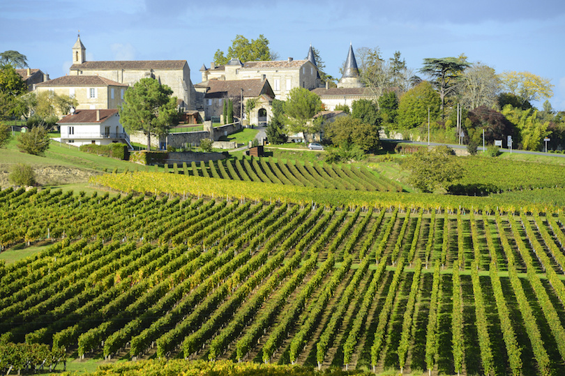
No doubt many of you sharp-eyed readers will have spotted a spelling error, thinking I intended to refer to one of these:

Fig 1


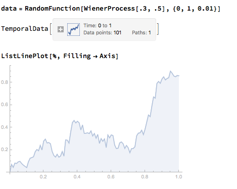
But, in fact, I really did have in mind something more like this:


wine pour


We are following an example from the recently published Mathematica Beyond Mathematics by Jose Sanchez Leon, an up-to-date text that describes many of the latest features in Mathematica, illustrated with interesting applications. Sanchez Leon shows how Mathematica’s machine learning capabilities can be applied to the craft of wine-making.

SSALGOTRADING AD

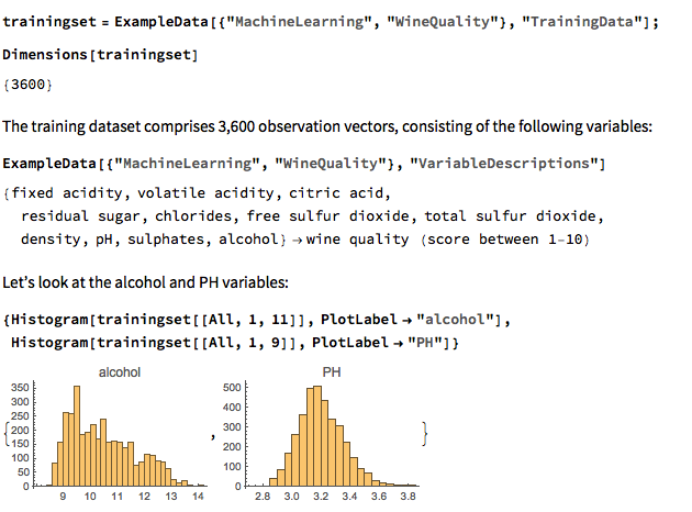
We begin by loading a curated Wolfram dataset comprising measurements of the physical properties and quality of wines:

Fig 2

A Machine Learning Prediction Model for Wine Quality

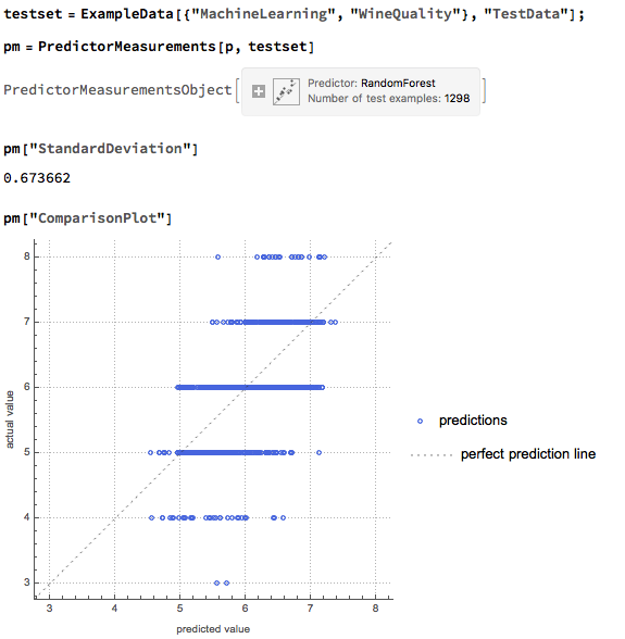
We’re going to apply Mathematica’s built-in machine learning algorithms to train a predictor of wine quality, using the training dataset. Mathematica determines that the most effective machine learning technique in this case is Random Forest and after a few seconds produces the predictor function:

Fig 3


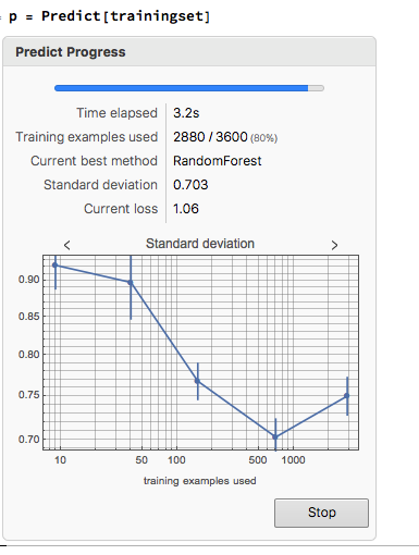
Mathematica automatically selects what it considers to be the best performing model from several available machine learning algorithms:

machine learning methods

Let’s take a look at how well the predictor perform on the test dataset of 1,298 wines:

Fig 4

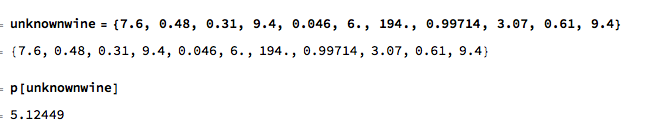
We can use the predictor function to predict the quality of an unknown wine, based on its physical properties:

Fig 5

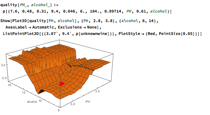
Next we create a function to predict the quality of an unknown wine as a function of just two of its characteristics, its pH and alcohol level.  The analysis suggests that the quality of our unknown wine could be improved by increasing both its pH and alcohol content:

Fig 6

Applications and Examples

This simple toy example illustrates how straightforward it is to deploy machine learning techniques in Mathematica.  Machine Learning and Neural Networks became a major focus for Wolfram Research in version 10, and the software’s capabilities have been significantly enhanced in version 11, with several applications such as text and sentiment analysis that have direct relevance to trading system development:

Fig 7

For other detailed examples see:

http://jonathankinlay.com/2016/08/machine-learning-model-spy/

http://jonathankinlay.com/2016/11/trading-market-sentiment/


http://jonathankinlay.com/2016/08/dynamic-time-warping/


Correlation Copulas

Continuing a previous post, in which we modeled the relationship in the levels of the VIX Index and the Year 1 and Year 2 CBOE Correlation Indices, we next turn our attention to modeling changes in the VIX index.

In case you missed it, the post can be found here:

http://jonathankinlay.com/2017/08/correlation-cointegration/

We saw previously that the levels of the three indices are all highly correlated, and we were able to successfully account for approximately half the variation in the VIX index using either linear regression models or non-linear machine-learning models that incorporated the two correlation indices.  It turns out that the log-returns processes are also highly correlated:

Fig1 Fig2

A Linear Model of VIX Returns

We can create a simple linear regression model that relates log-returns in the VIX index to contemporaneous log-returns in the two correlation indices, as follows.  The derived model accounts for just under 40% of the variation in VIX index returns, with each correlation index contributing approximately one half of the total VIX return.

SSALGOTRADING AD

Fig3

Non-Linear Model of VIX Returns

Although the linear model is highly statistically significant, we see clear evidence of lack of fit in the model residuals, which indicates non-linearities present in the relationship.  So, ext we use a nearest-neighbor algorithm, a machine learning technique that allows us to model non-linear components of the relationship.  The residual plot from the nearest neighbor model clearly shows that it does a better job of capturing these nonlinearities, with lower standard in the model residuals, compared to the linear regression model:

Fig4

Correlation Copulas

Another approach entails the use of copulas to model the inter-dependency between the volatility and correlation indices.  For a fairly detailed exposition on copulas, see the following blog posts:

http://jonathankinlay.com/2017/01/copulas-risk-management/


http://jonathankinlay.com/2017/03/pairs-trading-copulas/

We begin by taking a smaller sample comprising around three years of daily returns in the indices.  This minimizes the impact of any long-term nonstationarity in the processes and enables us to fit marginal distributions relatively easily.  First, let’s look at the correlations in our sample data:

Fig5

We next proceed to fit margin distributions to the VIX and Correlation Index processes.  It turns out that the VIX process is well represented by a Logistic distribution, while the two Correlation Index returns processes are better represented by a Student-T density.  In all three cases there is little evidence of lack of fit, wither in the body or tails of the estimated probability density functions:

Fig6 Fig7 Fig8

The final step is to fit a copula to model the joint density between the indices.  To keep it simple I have chosen to carry out the analysis for the combination of the VIX index with only the first of the correlation indices, although in principle there no reason why a copula could not be estimated for all three indices.  The fitted model is a multinormal Gaussian copula with correlation coefficient of 0.69.  of course, other copulas are feasible (Clayton, Gumbel, etc), but Gaussian model appears to provide an adequate fit to the empirical copula, with approximate symmetry in the left and right tails.

Fig9


A Tactical Equity Strategy

We have created a long-only equity strategy that aims to beat the S&P 500 total return benchmark by using tactical allocation algorithms to invest in equity ETFs.   One of the principal goals of the strategy is to protect investors’ capital during periods of severe market stress such as in the downturns of 2000 and 2008.  The strategy times the allocation of capital to equity ETFs or short-duration Treasury securities when investment opportunities are limited.

SSALGOTRADING AD

Systematic Strategies is a hedge fund rather than an RIA, so we have no plans to offer the product to the public.  However, we are currently holding exploratory discussions with Registered Investment Advisors about how the strategy might be made available to their clients.

For more background, see this post on Seeking Alpha: http://tiny.cc/ba3kny


Slide1


Slide2