October 2020 - QUANTITATIVE RESEARCH AND TRADING

October 27, 2020

On Testing Direction Prediction Accuracy

As regards the question of forecasting accuracy discussed in the paper on Forecasting Volatility in the S&P 500 Index, there are two possible misunderstandings here that need to be cleared up. These arise from remarks by one commentator as follows:

“An above 50% vol direction forecast looks good,.. but “direction” is biased when working with highly skewed distributions! ..so it would be nice if you could benchmark it against a simple naive predictors to get a feel for significance, -or- benchmark it with a trading strategy and see how the risk/return performs.”

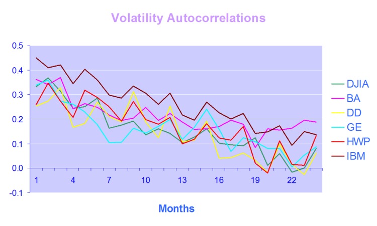
(i) The first point is simple, but needs saying: the phrase “skewed distributions” in the context of volatility modeling could easily be misconstrued as referring to the volatility skew. This, of course, is used to describe to the higher implied vols seen in the Black-Scholes prices of OTM options. But in the Black-Scholes framework volatility is constant, not stochastic, and the “skew” referred to arises in the distribution of the asset return process, which has heavier tails than the Normal distribution (excess Kurtosis and/or skewness). I realize that this is probably not what the commentator meant, but nonetheless it’s worth heading that possible misunderstanding off at the pass, before we go on.

(ii) I assume that the commentator was referring to the skewness in the volatility process, which is characterized by the LogNormal distribution. But the forecasting tests referenced in the paper are tests of the ability of the model to predict the direction of volatility, i.e. the sign of the change in the level of volatility from the current period to the next period. Thus we are looking at, not a LogNormal distribution, but the difference in two LogNormal distributions with equal mean – and this, of course, has an expectation of zero. In other words, the expected level of volatility for the next period is the same as the current period and the expected change in the level of volatility is zero. You can test this very easily for yourself by generating a large number of observations from a LogNormal process, taking the difference and counting the number of positive and negative changes in the level of volatility from one period to the next. You will find, on average, half the time the change of direction is positive and half the time it is negative.

For instance, the following chart shows the distribution of the number of positive changes in the level of a LogNormally distributed random variable with mean and standard deviation of 0.5, for a sample of 1,000 simulations, each of 10,000 observations. The sample mean (5,000.4) is very close to the expected value of 5,000.

Distribution Number of Positive Direction Changes

So, a naive predictor will forecast volatility to remain unchanged for the next period and by random chance approximately half the time volatility will turn out to be higher and half the time it will turn out to be lower than in the current period. Hence the default probability estimate for a positive change of direction is 50% and you would expect to be right approximately half of the time. In other words, the direction prediction accuracy of the naive predictor is 50%. This, then, is one of the key benchmarks you use to assess the ability of the model to predict market direction. That is what test statistics like Theil’s-U does – measures the performance relative to the naive predictor. The other benchmark we use is the change of direction predicted by the implied volatility of ATM options.
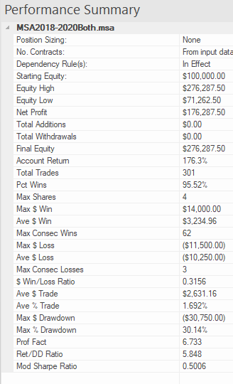
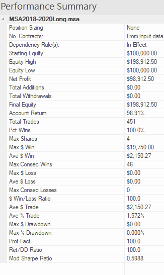
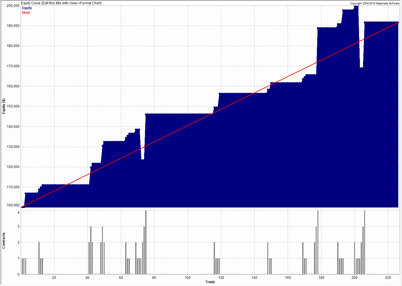
In this context, the model’s 61% or higher direction prediction accuracy is very significant (at the 4% level in fact) and this is reflected in the Theil’s-U statistic of 0.82 (lower is better). By contrast, Theil’s-U for the Implied Volatility forecast is 1.46, meaning that IV is a much worse predictor of 1-period-ahead changes in volatility than the naive predictor.

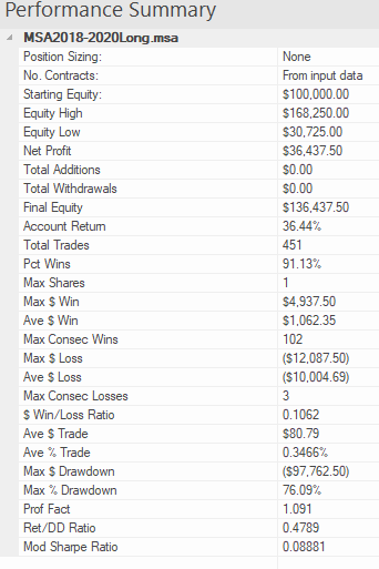
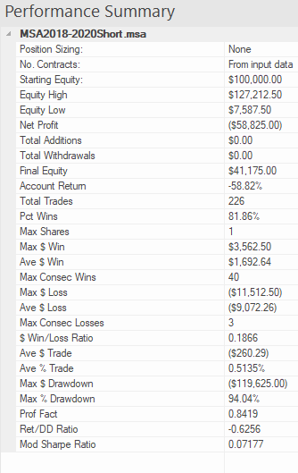
On its face, it is because of this exceptional direction prediction accuracy that a simple strategy is able to generate what appear to be abnormal returns using the change of direction forecasts generated by the model, as described in the paper. In fact, the situation is more complicated than that, once you introduce the concept of a market price of volatility risk.

October 20, 2020

Long Memory and Regime Shifts in Asset Volatility

This post covers quite a wide range of concepts in volatility modeling relating to long memory and regime shifts and is based on an article that was published in Wilmott magazine and republished in The Best of Wilmott Vol 1 in 2005. A copy of the article can be downloaded here.

One of the defining characteristics of volatility processes in general (not just financial assets) is the tendency for the serial autocorrelations to decline very slowly. This effect is illustrated quite clearly in the chart below, which maps the autocorrelations in the volatility processes of several financial assets.

Thus we can say that events in the volatility process for IBM, for instance, continue to exert influence on the process almost two years later.

This feature in one that is typical of a black noise process – not some kind of rap music variant, but rather:

“a process with a 1/f^β spectrum, where β > 2 (Manfred Schroeder, “Fractals, chaos, power laws“). Used in modeling various environmental processes. Is said to be a characteristic of “natural and unnatural catastrophes like floods, droughts, bear markets, and various outrageous outages, such as those of electrical power.” Further, “because of their black spectra, such disasters often come in clusters.”” [Wikipedia].

Because of these autocorrelations, black noise processes tend to reinforce or trend, and hence (to some degree) may be forecastable. This contrasts with a white noise process, such as an asset return process, which has a uniform power spectrum, insignificant serial autocorrelations and no discernable trending behavior:

An econometrician might describe this situation by saying that a black noise process is fractionally integrated order d, where d = H/2, H being the Hurst Exponent. A way to appreciate the difference in the behavior of a black noise process vs. a white process is by comparing two fractionally integrated random walks generated using the same set of quasi random numbers by Feder’s (1988) algorithm (see p 32 of the presentation on Modeling Asset Volatility).

Fractal Random Walk - White Noise — Fractal Random Walk – White Noise

Fractal Random Walk - Black Noise Process — Fractal Random Walk – Black Noise Process

As you can see. both random walks follow a similar pattern, but the black noise random walk is much smoother, and the downward trend is more clearly discernible. You can play around with the Feder algorithm, which is coded in the accompanying Excel Workbook on Volatility and Nonlinear Dynamics . Changing the Hurst Exponent parameter H in the worksheet will rerun the algorithm and illustrate a fractal random walk for a black noise (H > 0.5), white noise (H=0.5) and mean-reverting, pink noise (H<0.5) process.

One way of modeling the kind of behavior demonstrated by volatility process is by using long memory models such as ARFIMA and FIGARCH (see pp 47-62 of the Modeling Asset Volatility presentation for a discussion and comparison of various long memory models). The article reviews research into long memory behavior and various techniques for estimating long memory models and the coefficient of fractional integration d for a process.

But long memory is not the only possible cause of long term serial correlation. The same effect can result from structural breaks in the process, which can produce spurious autocorrelations. The article goes on to review some of the statistical procedures that have been developed to detect regime shifts, due to Bai (1997), Bai and Perron (1998) and the Iterative Cumulative Sums of Squares methodology due to Aggarwal, Inclan and Leal (1999). The article illustrates how the ICSS technique accurately identifies two changes of regimes in a synthetic GBM process.

In general, I have found the ICSS test to be a simple and highly informative means of gaining insight about a process representing an individual asset, or indeed an entire market. For example, ICSS detects regime shifts in the process for IBM around 1984 (the time of the introduction of the IBM PC), the automotive industry in the early 1980’s (Chrysler bailout), the banking sector in the late 1980’s (Latin American debt crisis), Asian sector indices in Q3 1997, the S&P 500 index in April 2000 and just about every market imaginable during the 2008 credit crisis. By splitting a series into pre- and post-regime shift sub-series and examining each segment for long memory effects, one can determine the cause of autocorrelations in the process. In some cases, Asian equity indices being one example, long memory effects disappear from the series, indicating that spurious autocorrelations were induced by a major regime shift during the 1997 Asian crisis. In most cases, however, long memory effects persist.

Excel Workbook on Volatility and Nonlinear Dynamics

There are several other topics from chaos theory and nonlinear dynamics covered in the workbook, including:

Generation of the Sierpinski triangle
Estimation of the Hurst Exponent in various series (Industrial Production, DJIA, S&P500)
Logistic and Henon attractors
Estimation of the fractal dimension and correlation integral for the S&P500 index

Modeling Asset Volatility

I am planning a series of posts on the subject of asset volatility and option pricing and thought I would begin with a survey of some of the central ideas. The attached presentation on Modeling Asset Volatility sets out the foundation for a number of key concepts and the basis for the research to follow.

Perhaps the most important feature of volatility is that it is stochastic rather than constant, as envisioned in the Black Scholes framework. The presentation addresses this issue by identifying some of the chief stylized facts about volatility processes and how they can be modelled. Certain characteristics of volatility are well known to most analysts, such as, for instance, its tendency to “cluster” in periods of higher and lower volatility. However, there are many other typical features that are less often rehearsed and these too are examined in the presentation.

Long Memory
For example, while it is true that GARCH models do a fine job of modeling the clustering effect they typically fail to capture one of the most important features of volatility processes – long term serial autocorrelation. In the typical GARCH model autocorrelations die away approximately exponentially, and historical events are seen to have little influence on the behaviour of the process very far into the future. In volatility processes that is typically not the case, however: autocorrelations die away very slowly and historical events may continue to affect the process many weeks, months or even years ahead.

Volatility Direction Prediction Accuracy

There are two immediate and very important consequences of this feature. The first is that volatility processes will tend to trend over long periods – a characteristic of Black Noise or Fractionally Integrated processes, compared to the White Noise behavior that typically characterizes asset return processes. Secondly, and again in contrast with asset return processes, volatility processes are inherently predictable, being conditioned to a significant degree on past behavior. The presentation considers the fractional integration frameworks as a basis for modeling and forecasting volatility.

Mean Reversion vs. Momentum
A puzzling feature of much of the literature on volatility is that it tends to stress the mean-reverting behavior of volatility processes. This appears to contradict the finding that volatility behaves as a reinforcing process, whose long-term serial autocorrelations create a tendency to trend. This leads to one of the most important findings about asset processes in general, and volatility process in particular: i.e. that the assets processes are simultaneously trending and mean-reverting. One way to understand this is to think of volatility, not as a single process, but as the superposition of two processes: a long term process in the mean, which tends to reinforce and trend, around which there operates a second, transient process that has a tendency to produce short term spikes in volatility that decay very quickly. In other words, a transient, mean reverting processes inter-linked with a momentum process in the mean. The presentation discusses two-factor modeling concepts along these lines, and about which I will have more to say later.

Cointegration
One of the most striking developments in econometrics over the last thirty years, cointegration is now a principal weapon of choice routinely used by quantitative analysts to address research issues ranging from statistical arbitrage to portfolio construction and asset allocation. Back in the late 1990’s I and a handful of other researchers realized that volatility processes exhibited very powerful cointegration tendencies that could be harnessed to create long-short volatility strategies, mirroring the approach much beloved by equity hedge fund managers. In fact, this modeling technique provided the basis for the Caissa Capital volatility fund, which I founded in 2002. The presentation examines characteristics of multivariate volatility processes and some of the ideas that have been proposed to model them, such as FIGARCH (fractionally-integrated GARCH).

Dispersion Dynamics
Finally, one topic that is not considered in the presentation, but on which I have spent much research effort in recent years, is the behavior of cross-sectional volatility processes, which I like to term dispersion. It turns out that, like its univariate cousin, dispersion displays certain characteristics that in principle make it highly forecastable. Given an appropriate model of dispersion dynamics, the question then becomes how to monetize efficiently the insight that such a model offers. Again, I will have much more to say on this subject, in future.

October 7, 2020

A Meta-Strategy in S&P 500 E-Mini Futures

In earlier posts I have described the idea of a meta-strategy as a strategies that trades strategies. It is an algorithm, or set of rules, that is used to decide when to trade an underlying strategy. In some cases a meta-strategy may influence the size in which the underlying strategy is traded, or may even amend the base code. In other word, a meta-strategy actively “trades” an underlying strategy, or group of strategies, much as in the same way a regular strategy may actively trade stocks, going long or short from time to time. One distinction is that a meta-strategy will rarely, if ever, actually “short” an underlying strategy – at most it will simply turn the strategy off (reduce the position size to zero) for a period.

For a more detailed description, see this post:

Improving Trading System Performance Using a Meta-Strategy

In this post I look at a meta-strategy that developed for a client’s strategy in S&P E-Mini futures. What is extraordinary is that the underlying strategy was so badly designed (not by me!) and performs so poorly that no rational systematic trader would likely give it a second look – instead he would toss it into the large heap of failed ideas that all quantitative researchers accumulate over the course of their careers. So this is a textbook example that illustrates the power of meta-strategies to improve, or in this case transform, the performance of an underlying strategy.

1. The Strategy

The Target Trader Strategy (“TTS”) is a futures strategy applied to S&P 500 E-Mini futures that produces a very high win rate, but which occasionally experiences very large losses. The purpose of the analysis if to find methods that will:

1) Decrease the max loss / drawdown
2) Increase the win rate / profitability

For longs the standard setting is entry 40 ticks below the target, stop loss 1000 ticks below the target, and then 2 re-entries 100 ticks below entry 1 and 100 ticks below entry 2

For shorts the standard is entry 80 ticks above the target. stop loss 1000 ticks above the target, and then 2 re-entries 100 ticks above entry 1 and 100 ticks above entry 2

For both directions its 80 ticks above/below for entry 1, 1000 tick stop, and then 1 re entry 100 ticks above/below, and then re-entry 2 100 ticks above/below entry 2

2. Strategy Performance

2.1 Overall Performance

The overall performance of the strategy over the period from 2018 to 2020 is summarized in the chart of the strategy equity curve and table of performance statistics below.
These confirm that, while the win rate if very high (over 84%) there strategy experiences many significant drawdowns, including a drawdown of -$61,412.50 (-43.58%). The total return is of the order of 5% per year, the strategy profit factor is fractionally above 1 and the Sharpe Ratio is negligibly small. Many traders would consider the performance to be highly unattractive.

2.2 Long Trades

We break the strategy performance down into long and short trades, and consider them separately. On the long side, the strategy has been profitable, producing a gain of over 36% during the period 2018-2020. It also suffered catastrophic drawdown of over -$97,000 during that period:

2.3 Short Trades

On the short side, the story is even worse, producing an overall loss of nearly -$59,000:

3. Improving Strategy Performance with a Meta-Strategy

We considered two possible methods to improve strategy performance. The first method attempts to apply technical indicators and other data series to improve trading performance. Here we evaluated price series such as the VIX index and a wide selection of technical indicators, including RSI, ADX, Moving Averages, MACD, ATR and others. However, any improvement in strategy performance proved to be temporary in nature and highly variable, in many cases amplifying the problems with the strategy performance rather than improving them.

The second approach proved much more effective, however. In this method we create a meta-strategy which effectively “trades the strategy”, turning it on and off depending on its recent performance. The meta-strategy consists of a set of rules that determines whether or not to continue trading the strategy after a series of wins or losses. In some cases the meta-strategy may increase the trade size for a sequence of trades, at times when it considers the conditions for the underlying strategy to be favorable.

The result of applying the meta-strategy are described in the following sections.

3.1 Long & Short Strategies with Meta-Strategy Overlay

The performance of the long/short strategies combined with the meta-strategy overlay are set out in the chart and table below.
The overall improvements can be summarized as follows:

Net profit increases from $15,387 to $176,287
Account return rises from 15% to 176%
Percentage win rate rises from 84% to 95%
Profit factor increases from 1.0 to 6.7
Average trade rises from $51 to $2,631
Max $ Drawdown falls from -$61,412 to -$30,750
Return/Max Drawdown ratio rises from 0.35 to 5.85
The modified Sharpe ratio increases from 0.07 to 0.5

Taken together, these are dramatic improvements to every important aspect of strategy performance.

There are two key rules in the meta-strategy, applicable to winning and losing trades:

Rule for winning trades:
After 3 wins in a row, skip the next trade.

Rule for losing trades:
After 3 losses in a row, add 1 contract until the first win. Subtract 1 contract after each win until the next loss, or back to 1 contract.

3.2 Long Trades with Meta-Strategy

The meta-strategy rules produce significant improvements in the performance of both the long and short components of the strategy. On the long side the percentage win rate is increased to 100% and the max % drawdown is reduced to 0%:

3.3 Short Trades with Meta-Strategy

Improvements to the strategy on the short side are even more significant, transforming a loss of -$59,000 into a profit of $91,600:

4. Conclusion

A meta-strategy is a simple, yet powerful technique that can transform the performance of an underlying strategy. The rules are often simple, although they can be challenging to implement. Meta strategies can be applied to almost any underlying strategy, whether in futures, equities, or forex. Worthwhile improvements in strategy performance are often achievable, although not often as spectacular as in this case.

If any reader is interested in designing a meta-strategy for their own use, please get in contact.

October 6, 2020

Market Timing in the S&P 500 Index Using Volatility Forecasts

There has been a good deal of interest in the market timing ideas discussed in my earlier blog post Using Volatility to Predict Market Direction, which discusses the research of Diebold and Christoffersen into the sign predictability induced by volatility dynamics. The ideas are thoroughly explored in a QuantNotes article from 2006, which you can download here.

There is a follow-up article from 2006 in which Christoffersen, Diebold, Mariano and Tay develop the ideas further to consider the impact of higher moments of the asset return distribution on sign predictability and the potential for market timing in international markets (download here).

Trading Strategy
To illustrate some of the possibilities of this approach, we constructed a simple market timing strategy in which a position was taken in the S&P 500 index or in 90-Day T-Bills, depending on an ex-ante forecast of positive returns from the logit regression model (and using an expanding window to estimate the drift coefficient). We assume that the position is held for 30 days and rebalanced at the end of each period. In this test we make no allowance for market impact, or transaction costs.

Results
Annual returns for the strategy and for the benchmark S&P 500 Index are shown in the figure below. The strategy performs exceptionally well in 1987, 1989 and 1995, when the ratio between expected returns and volatility remains close to optimum levels and the direction of the S&P 500 Index is highly predictable, Of equal interest is that the strategy largely avoids the market downturn of 2000-2002 altogether, a period in which sign probabilities were exceptionally low.

In terms of overall performance, the model enters the market in 113 out of a total of 241 months (47%) and is profitable in 78 of them (69%). The average gain is 7.5% vs. an average loss of –4.11% (ratio 1.83). The compound annual return is 22.63%, with an annual volatility of 17.68%, alpha of 14.9% and Sharpe ratio of 1.10.

The under-performance of the strategy in 2003 is explained by the fact that direction-of-change probabilities were rising from a very low base in Q4 2002 and do not reach trigger levels until the end of the year. Even though the strategy out-performed the Index by a substantial margin of 6% , the performance in 2005 is of concern as market volatility was very low and probabilities overall were on a par with those seen in 1995. Further tests are required to determine whether the failure of the strategy to produce an exceptional performance on par with 1995 was the result of normal statistical variation or due to changes in the underlying structure of the process requiring model recalibration.

Future Research & Development
The obvious next step is to develop the approach described above to formulate trading strategies based on sign forecasting in a universe of several assets, possibly trading binary options. The approach also has potential for asset allocation, portfolio theory and risk management applications.