A Practical Application of Regime Switching Models to Pairs Trading

In the previous post I outlined some of the available techniques used for modeling market states.  The following is an illustration of how these techniques can be applied in practice.    You can download this post in pdf format here.

SSALGOTRADING AD

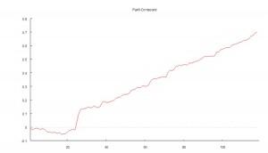
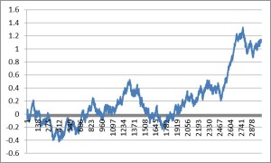
The chart below shows the daily compounded returns for a single pair in an ETF statistical arbitrage strategy, back-tested over a 1-year period from April 2010 to March 2011.

The idea is to examine the characteristics of the returns process and assess its predictability.

Pairs Trading

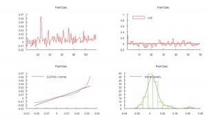
The initial impression given by the analytics plots of daily returns, shown in Fig 2 below, is that the process may be somewhat predictable, given what appears to be a significant 1-order lag in the autocorrelation spectrum.  We also see evidence of the
customary non-Gaussian “fat-tailed” distribution in the error process.

Regime Switching

An initial attempt to fit a standard Auto-Regressive Moving Average ARMA(1,0,1) model  yields disappointing results, with an unadjusted  model R-squared of only 7% (see model output in Appendix 1)

However, by fitting a 2-state Markov model we are able to explain as much as 65% in the variation in the returns process (see Appendix II).
The model estimates Markov Transition Probabilities as follows.

P(.|1)       P(.|2)

P(1|.)       0.93920      0.69781

P(2|.)     0.060802      0.30219

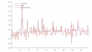
In other words, the process spends most of the time in State 1, switching to State 2 around once a month, as illustrated in Fig 3 below.

Markov model
In the first state, the  pairs model produces an expected daily return of around 65bp, with a standard deviation of similar magnitude.  In this state, the process also exhibits very significant auto-regressive and moving average features.

Regime 1:

Intercept                   0.00648     0.0009       7.2          0

AR1                            0.92569    0.01897   48.797        0

MA1                         -0.96264    0.02111   -45.601        0

Error Variance^(1/2)           0.00666     0.0007

In the second state, the pairs model  produces lower average returns, and with much greater variability, while the autoregressive and moving average terms are poorly determined.

Regime 2:

Intercept                    0.03554    0.04778    0.744    0.459

AR1                            0.79349    0.06418   12.364        0

MA1                         -0.76904    0.51601     -1.49   0.139

Error Variance^(1/2)           0.01819     0.0031

CONCLUSION
The analysis in Appendix II suggests that the residual process is stable and Gaussian.  In other words, the two-state Markov model is able to account for the non-Normality of the returns process and extract the salient autoregressive and moving average features in a way that makes economic sense.

How is this information useful?  Potentially in two ways:

(i)     If the market state can be forecast successfully, we can use that information to increase our capital allocation during periods when the process is predicted to be in State 1, and reduce the allocation at times when it is in State 2.

(ii)    By examining the timing of the Markov states and considering different features of the market during the contrasting periods, we might be able to identify additional explanatory factors that could be used to further enhance the trading model.

Markov model

Regime-Switching & Market State Modeling

The Excel workbook referred to in this post can be downloaded here.

Market state models are amongst the most useful analytical techniques that can be helpful in developing alpha-signal generators.  That term covers a great deal of ground, with ideas drawn from statistics, econometrics, physics and bioinformatics.  The purpose of this short note is to provide an introduction to some of the key ideas and suggest ways in which they might usefully applied in the context of researching and developing trading systems.

Although they come from different origins, the concepts presented here share common foundational principles:

  1. Markets operate in different states that may be characterized by various measures (volatility, correlation, microstructure, etc);
  2. Alpha signals can be generated more effectively by developing models that are adapted to take account of different market regimes;
  3. Alpha signals may be combined together effectively by taking account of the various states that a market may be in.

Market state models have shown great promise is a variety of applications within the field of applied econometrics in finance, not only for price and market direction forecasting, but also basis trading, index arbitrage, statistical arbitrage, portfolio construction, capital allocation and risk management.

REGIME SWITCHING MODELS

These are econometric models which seek to use statistical techniques to characterize market states in terms of different estimates of the parameters of some underlying linear model.  This is accompanied by a transition matrix which estimates the probability of moving from one state to another.

To illustrate this approach I have constructed a simple example, given in the accompanying Excel workbook.  In this model the market operates as follows:

econometric Where

Yt is a variable of interest (e.g. the return in an asset over the next period t) 

et is an error process with constant variance s2 

S is the market state, with two regimes (S=1 or S=2) 

a0 is the drift in the asset process 

a1 is an autoregressive term, by which the return in the current period is dependent on the prior period return 

b1 is a moving average term, which smoothes the error process 

 This is one of the simplest possible structures, which in more general form can include multiple states, and independent regressions Xi as explanatory variables (such as book pressure, order flow, etc):

econometric


SSALGOTRADING AD

The form of the error process et may also be dependent on the market state.  It may simply be that, as in this example, the standard deviation of the error process changes from state to state.  But the changes can also be much more complex:  for instance, the error process may be non-Gaussian, or it may follow a formulation from the GARCH framework.

In this example the state parameters are as follows:

Reg1 Reg 2
s 0.01 0.02
a0 0.005 -0.015
a1 0.40 0.70
b1 0.10 0.20

What this means is that, in the first state the market tends to trend upwards with relatively low volatility.  In the second state, not only is market volatility much higher, but also the trend is 3x as large in the negative direction.

I have specified the following state transition matrix:

Reg1 Reg2
Reg1 0.85 0.15
Reg2 0.90 0.10

This is interpreted as follows:  if the market is in State 1, it will tend to remain in that state 85% of the time, transitioning to State 2 15% of the time.  Once in State 2, the market tends to revert to State 1 very quickly, with 90% probability.  So the system is in State 1 most of the time, trending slowly upwards with low volatility and occasionally flipping into an aggressively downward trending phase with much higher volatility.

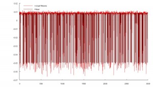
The Generate sheet in the Excel workbook shows how observations are generated from this process, from which we select a single instance of 3,000 observations, shown in sheet named Sample.

The sample looks like this:


Market state 


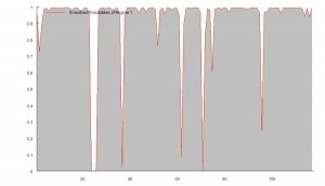
 As anticipated, the market is in State 1 most of the time, occasionally flipping into State 2 for brief periods.
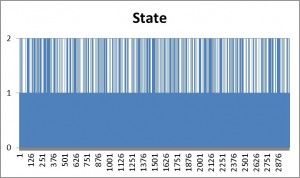
Market state 

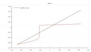
 It is well-known that in financial markets we are typically dealing with highly non-Gaussian distributions.  Non-Normality can arise for a number of reasons, including changes in regimes, as illustrated here.  It is worth noting that, even though in this example the process in either market state follows a Gaussian distribution, the combined process is distinctly non-Gaussian in form, having (extremely) fat tails, as shown by the QQ-plot below.
 

 Market state

If we attempt to fit a standard ARMA model to the process, the outcome is very disappointing in terms of the model’s poor explanatory power (R2 0.5%) and lack of fit in the squared-residuals:


ARIMA(1,0,1)

         Estimate  Std. Err.   t Ratio  p-Value

Intercept                      0.00037    0.00032     1.164    0.244

AR1                            0.57261     0.1697     3.374    0.001

MA1                           -0.63292    0.16163    -3.916        0

Error Variance^(1/2)           0.02015     0.0004    ——   ——

                       Log Likelihood = 7451.96

                    Schwarz Criterion = 7435.95

               Hannan-Quinn Criterion = 7443.64

                     Akaike Criterion = 7447.96

                       Sum of Squares =  1.2172

                            R-Squared =  0.0054

                        R-Bar-Squared =  0.0044

                          Residual SD =  0.0202

                    Residual Skewness = -2.1345

                    Residual Kurtosis =  5.7279

                     Jarque-Bera Test = 3206.15     {0}

Box-Pierce (residuals):         Q(48) = 59.9785 {0.115}

Box-Pierce (squared residuals): Q(50) = 78.2253 {0.007}

              Durbin Watson Statistic = 2.01392

                    KPSS test of I(0) =  0.2001    {<1} *

                 Lo’s RS test of I(0) =  1.2259  {<0.5} *

Nyblom-Hansen Stability Test:  NH(4)  =  0.5275    {<1}

MA form is 1 + a_1 L +…+ a_q L^q.

Covariance matrix from robust formula.

* KPSS, RS bandwidth = 0.

Parzen HAC kernel with Newey-West plug-in bandwidth.


However, if we keep the same simple form of ARMA(1,1) model, but allow for the possibility of a two-state Markov process, the picture alters dramatically:  now the model is able to account for 98% of the variation in the process, as shown below.


Notice that we have succeeded in estimating the correct underlying transition probabilities, and how the ARMA model parameters change from regime to regime much as they should (small positive drift in one regime, large negative drift in the second, etc).


Markov Transition Probabilities

                    P(.|1)       P(.|2)

P(1|.)            0.080265      0.14613

P(2|.)             0.91973      0.85387


                              Estimate  Std. Err.   t Ratio  p-Value

Logistic, t(1,1)              -2.43875     0.1821    ——   ——

Logistic, t(1,2)              -1.76531     0.0558    ——   ——

Non-switching parameters shown as Regime 1.


Regime 1:

Intercept                     -0.05615    0.00315   -17.826        0

AR1                            0.70864    0.16008     4.427        0

MA1                           -0.67382    0.16787    -4.014        0

Error Variance^(1/2)           0.00244     0.0001    ——   ——


Regime 2:

Intercept                      0.00838     2e-005   419.246        0

AR1                            0.26716    0.08347     3.201    0.001

MA1                           -0.26592    0.08339    -3.189    0.001


                       Log Likelihood = 12593.3

                    Schwarz Criterion = 12557.2

               Hannan-Quinn Criterion = 12574.5

                     Akaike Criterion = 12584.3

                       Sum of Squares =  0.0178

                            R-Squared =  0.9854

                        R-Bar-Squared =  0.9854

                          Residual SD =  0.002

                    Residual Skewness = -0.0483

                    Residual Kurtosis = 13.8765

                     Jarque-Bera Test = 14778.5     {0}

Box-Pierce (residuals):         Q(48) = 379.511     {0}

Box-Pierce (squared residuals): Q(50) = 36.8248 {0.917}

              Durbin Watson Statistic = 1.50589

                    KPSS test of I(0) =  0.2332    {<1} *

                 Lo’s RS test of I(0) =  2.1352 {<0.005} *

Nyblom-Hansen Stability Test:  NH(9)  =  0.8396    {<1}

MA form is 1 + a_1 L +…+ a_q L^q.

Covariance matrix from robust formula.

* KPSS, RS bandwidth = 0.

Parzen HAC kernel with Newey-West plug-in bandwidth.

regime switching

There are a variety of types of regime switching mechanisms we can use in state models:


Hamiltonian – the simplest, where the process mean and variance vary from state to state

Markovian – the approach used here, with state transition matrix

Explained Switching – where the process changes state as a result of the influence of some underlying variable (such as interest rate volatility, for example)

Smooth Transition – comparable to explained Markov switching, but without and explicitly probabilistic interpretation.


This example is both rather simplistic and pathological at the same time:  the states are well-separated , by design, whereas for real processes they tend to be much harder to distinguish.  A difficulty of this methodology is that the models can be very difficult to estimate.  The likelihood function tends to be very flat and there are a great many local maxima that give similar fit, but with widely varying model forms and parameter estimates.  That said, this is a very rich class of models with a great many potential applications.
Volatility Forecasting in Emerging Markets

The great majority of empirical studies have focused on asset markets in the US and other developed economies.   The purpose of this research is to determine to what extent the findings of other researchers in relation to the characteristics of asset volatility in developed economies applies also to emerging markets.  The important characteristics observed in asset volatility that we wish to identify and examine in emerging markets include clustering, (the tendency for periodic regimes of high or low volatility) long memory, asymmetry, and correlation with the underlying returns process.  The extent to which such behaviors are present in emerging markets will serve to confirm or refute the conjecture that they are universal and not just the product of some factors specific to the intensely scrutinized, and widely traded developed markets.

The ten emerging markets we consider comprise equity markets in Australia, Hong Kong, Indonesia, Malaysia, New Zealand, Philippines, Singapore, South Korea, Sri Lanka and Taiwan focusing on the major market indices for those markets.   After analyzing the characteristics of index volatility for these indices, the research goes on to develop single- and two-factor REGARCH models in the form by Alizadeh, Brandt and Diebold (2002).

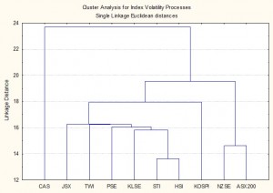
Cluster Analysis of Volatility
Processes for Ten Emerging Market Indices

The research confirms the presence of a number of typical characteristics of volatility processes for emerging markets that have previously been identified in empirical research conducted in developed markets.  These characteristics include volatility clustering, long memory, and asymmetry.   There appears to be strong evidence of a region-wide regime shift in volatility processes during the Asian crises in 1997, and a less prevalent regime shift in September 2001. We find evidence from multivariate analysis that the sample separates into two distinct groups:  a lower volatility group comprising the Australian and New Zealand indices and a higher volatility group comprising the majority of the other indices.

SSALGOTRADING AD

Models developed within the single- and two-factor REGARCH framework of Alizadeh, Brandt and Diebold (2002) provide a good fit for many of the volatility series and in many cases have performance characteristics that compare favorably with other classes of models with high R-squares, low MAPE and direction prediction accuracy of 70% or more.   On the debit side, many of the models demonstrate considerable variation in explanatory power over time, often associated with regime shifts or major market events, and this is typically accompanied by some model parameter drift and/or instability.

Single equation ARFIMA-GARCH models appear to be a robust and reliable framework for modeling asset volatility processes, as they are capable of capturing both the short- and long-memory effects in the volatility processes, as well as GARCH effects in the kurtosis process.   The available procedures for estimating the degree of fractional integration in the volatility processes produce estimates that appear to vary widely for processes which include both short- and long- memory effects, but the overall conclusion is that long memory effects are at least as important as they are for volatility processes in developed markets.  Simple extensions to the single-equation models, which include regressor lags of related volatility series, add significant explanatory power to the models and suggest the existence of Granger-causality relationships between processes.

Extending the modeling procedures into the realm of models which incorporate systems of equations provides evidence of two-way Granger causality between certain of the volatility processes and suggests that are fractionally cointegrated, a finding shared with parallel studies of volatility processes in developed markets.

Download paper here.

Resources for Quantitative Analysts

Two of the smartest econometricians I know are Prof. Stephen Taylor of Lancaster University, and Prof. James Davidson of Exeter University.

I recall spending many profitable hours in the 1980’s with Stephen’s book Modelling Financial Time Series, which I am pleased to see has now been reprinted in a second edition.  For a long time this was the best available book on the topic and it remains a classic. It has been surpassed by very few books, one being Stephen’s later work Asset Price Dynamics, Volatility and Prediction.  This is a superb exposition, one that will repay close study.

James Davidson is one of the smartest minds in econometrics. Not only is his research of the highest caliber, he has somehow managed (in his spare time!) to develop one of the most advanced econometrics packages available.  Based on Jurgen Doornik’s Ox programming system, the Time Series Modelling package covers almost every conceivable model type, including regression models, ARIMA, ARFIMA and other single equation models, systems of equations, panel data models, GARCH and other heteroscedastic models and regime switching models, accompanied by very comprehensive statistical testing capabilities.  Furthermore, TSM is very well documented and despite being arguably the most advanced system of its kind it is inexpensive relative to alternatives.  James’s research output is voluminous and often highly complex.  His book, Econometric Theory, is an excellent guide to the state of the art, but not for the novice (or the faint hearted!).

Those looking for a kinder, gentler introduction to econometrics would do well to acquire a copy of Prof. Chris Brooks’s Introductory Econometrics for Finance. This covers most of the key ideas, from regression, through ARMA, GARCH, panel data models, cointegration, regime switching and volatility modeling.  Not only is the coverage comprehensive, Chris’s explanation of the concepts is delightfully clear and illustrated with interesting case studies which he analyzes using the EViews econometrics package.    Although not as advanced as TSM, EViews has everything that most quantitative analysts are likely to require in a modeling system and is very well suited to Chris’s teaching style.  Chris’s research output is enormous and covers a great many topics of interest to financial market analysts, in the same lucid style.

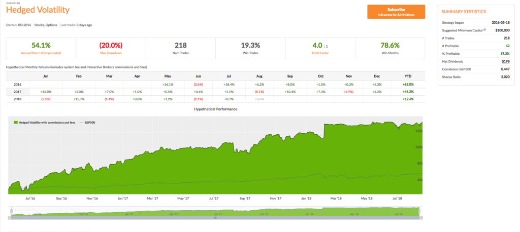
The Hedged Volatility Strategy

Being short regular Volatility ETFs or long Inverse Volatility ETFs are winning strategies…most of the time. The challenge is that when the VIX spikes or when the VIX futures curve is downward sloping instead of upward sloping, very significant losses can occur. Many people have built and back-tested models that attempt to move from long to short to neutral positions in the various Volatility ETFs, but almost all of them have one or both of these very significant flaws: 1) Failure to use “out of sample” back-testing and 2) Failure to protect against “black swan” events.

In this strategy a position and weighting in the appropriate Volatility ETFs are established based on a multi-factor model which always uses out of sample back-testing to determine effectiveness. Volatility Options are always used to protect against significant short-term moves which left unchecked could result in the total loss of one’s portfolio value; these options will usually lose money, but that is a small price to pay for the protection they provide. (Strategies should be scaled at a minimum of 20% to ensure options protection.)

This is a good strategy for IRA accounts in which short selling is not allowed. Long positions in Inverse Volatility ETFs are typically held. Suggested minimum capital: $26,000 (using 20% scaling).