A common theme of microstructure modeling is that trade flow is often predictive of market direction. One concept in particular that has gained traction is flow toxicity, i.e. flow where resting orders tend to be filled more quickly than expected, while aggressive orders rarely get filled at all, due to the participation of informed traders trading against uninformed traders. The fundamental insight from microstructure research is that the order arrival process is informative of subsequent price moves in general and toxic flow in particular. This is turn has led researchers to try to measure the probability of informed trading (PIN). One recent attempt to model flow toxicity, the Volume-Synchronized Probability of Informed Trading (VPIN)metric, seeks to estimate PIN based on volume imbalance and trade intensity. A major advantage of this approach is that it does not require the estimation of unobservable parameters and, additionally, updating VPIN in trade time rather than clock time improves its predictive power. VPIN has potential applications both in high frequency trading strategies, but also in risk management, since highly toxic flow is likely to lead to the withdrawal of liquidity providers, setting up the conditions for a flash-crash” type of market breakdown.
The procedure for estimating VPIN is as follows. We begin by grouping sequential trades into equal volume buckets of size V. If the last trade needed to complete a bucket was for a size greater than needed, the excess size is given to the next bucket. Then we classify trades within each bucket into two volume groups: Buys (V(t)B) and Sells (V(t)S), with V = V(t)B + V(t)S
The Volume-Synchronized Probability of Informed Trading is then derived as:
Typically one might choose to estimate VPIN using a moving average over n buckets, with n being in the range of 50 to 100.
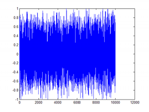
Another related statistic of interest is the single-period signed VPIN. This will take a value of between -1 and =1, depending on the proportion of buying to selling during a single period t.
Fig 1. Single-Period Signed VPIN for the ES Futures Contract
It turns out that quote revisions condition strongly on the signed VPIN. For example, in tests of the ES futures contract, we found that the change in the midprice from one volume bucket the next was highly correlated to the prior bucket’s signed VPIN, with a coefficient of 0.5. In other words, market participants offering liquidity will adjust their quotes in a way that directly reflects the direction and intensity of toxic flow, which is perhaps hardly surprising.
Of greater interest is the finding that there is a small but statistically significant dependency of price changes, as measured by first buy (sell) trade price to last sell (buy) trade price, on the prior period’s signed VPIN. The correlation is positive, meaning that strongly toxic flow in one direction has a tendency to push prices in the same direction during the subsequent period. Moreover, the single period signed VPIN turns out to be somewhat predictable, since its autocorrelations are statistically significant at two or more lags. A simple linear auto-regression ARMMA(2,1) model produces an R-square of around 7%, which is small, but statistically significant.
A more useful model, however , can be constructed by introducing the idea of Markov states and allowing the regression model to assume different parameter values (and error variances) in each state. In the Markov-state framework, the system transitions from one state to another with conditional probabilities that are estimated in the model.
An example of such a model for the signed VPIN in ES is shown below. Note that the model R-square is over 27%, around 4x larger than for a standard linear ARMA model.
We can describe the regime-switching model in the following terms. In the regime 1 state the model has two significant autoregressive terms and one significant moving average term (ARMA(2,1)). The AR1 term is large and positive, suggesting that trends in VPIN tend to be reinforced from one period to the next. In other words, this is a momentum state. In the regime 2 state the AR2 term is not significant and the AR1 term is large and negative, suggesting that changes in VPIN in one period tend to be reversed in the following period, i.e. this is a mean-reversion state.
The state transition probabilities indicate that the system is in mean-reversion mode for the majority of the time, approximately around 2 periods out of 3. During these periods, excessive flow in one direction during one period tends to be corrected in the
ensuring period. But in the less frequently occurring state 1, excess flow in one direction tends to produce even more flow in the same direction in the following period. This first state, then, may be regarded as the regime characterized by toxic flow.
Markov State Regime-Switching Model
Markov Transition Probabilities
P(.|1) P(.|2)
P(1|.) 0.54916 0.27782
P(2|.) 0.45084 0.7221
Regime 1:
AR1 1.35502 0.02657 50.998 0
AR2 -0.33687 0.02354 -14.311 0
MA1 0.83662 0.01679 49.828 0
Error Variance^(1/2) 0.36294 0.0058
Regime 2:
AR1 -0.68268 0.08479 -8.051 0
AR2 0.00548 0.01854 0.296 0.767
MA1 -0.70513 0.08436 -8.359 0
Error Variance^(1/2) 0.42281 0.0016
Log Likelihood = -33390.6
Schwarz Criterion = -33445.7
Hannan-Quinn Criterion = -33414.6
Akaike Criterion = -33400.6
Sum of Squares = 8955.38
R-Squared = 0.2753
R-Bar-Squared = 0.2752
Residual SD = 0.3847
Residual Skewness = -0.0194
Residual Kurtosis = 2.5332
Jarque-Bera Test = 553.472 {0}
Box-Pierce (residuals): Q(9) = 13.9395 {0.124}
Box-Pierce (squared residuals): Q(12) = 743.161 {0}
A Simple Trading Strategy
One way to try to monetize the predictability of the VPIN model is to use the forecasts to take directional positions in the ES
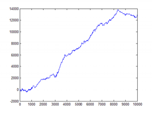
contract. In this simple simulation we assume that we enter a long (short) position at the first buy (sell) price if the forecast VPIN exceeds some threshold value 0.1 (-0.1). The simulation assumes that we exit the position at the end of the current volume bucket, at the last sell (buy) trade price in the bucket.
This simple strategy made 1024 trades over a 5-day period from 8/8 to 8/14, 90% of which were profitable, for a total of $7,675 – i.e. around ½ tick per trade.
The simulation is, of course, unrealistically simplistic, but it does give an indication of the prospects for more realistic version of the strategy in which, for example, we might rest an order on one side of the book, depending on our VPIN forecast.
Figure 2 – Cumulative Trade PL
References
Easley, D., Lopez de Prado, M., O’Hara, M., Flow Toxicity and Volatility in a High frequency World, Johnson School Research paper Series # 09-2011, 2011
Easley, D. and M. O‟Hara (1987), “Price, Trade Size, and Information in Securities Markets”, Journal of Financial Economics, 19.
Easley, D. and M. O‟Hara (1992a), “Adverse Selection and Large Trade Volume: The Implications for Market Efficiency”,
Journal of Financial and Quantitative Analysis, 27(2), June, 185-208.
Easley, D. and M. O‟Hara (1992b), “Time and the process of security price adjustment”, Journal of Finance, 47, 576-605.


