Intraday Stock Index Forecasting

In a previous post I discussed modelling stock prices processes as Geometric brownian Motion processes:

Understanding Stock Price Range Forecasts

To recap briefly, we assume a process of the form:

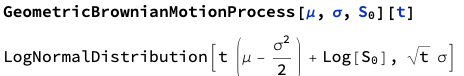
Where S0 is the initial stock price at time t = 0.

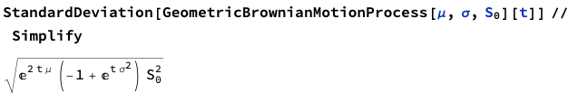
The mean of such a process is:

and standard deviation:

In the post I showed how to estimate such a process with daily stock prices, using these to provide a forecast range of prices over a one-month horizon. This is potentially useful, for example, in choosing which strikes to select in an option hedge.

Of course, there is nothing to prevent you from using the same technique over different timescales. Here I use the MATH-TWS package to connect Mathematica to the IB TWS platform via the C++ api, to extract intraday prices for the S&P 500 Index at 1-minute intervals. These are used to estimate a short-term GBM process, which provides forecasts of the mean and variance of the index at the 4 PM close.

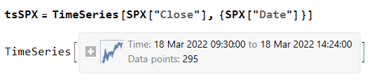
We capture the data using:

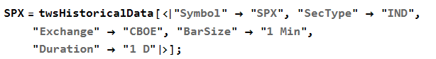
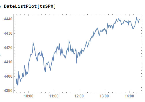
then create a time series of the intraday prices and plot them:

If we want something a little fancier we can create a trading chart, including technical indicators of our choice, for instance:

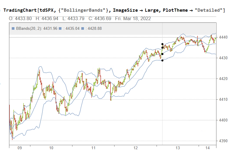
The charts can be updated in real time from IB, using MATHTWS.

From there we estimate a GBM process using 1-minute close prices:

and then simulate a number of price paths towards the 4 PM close (the mean price path is shown in black):

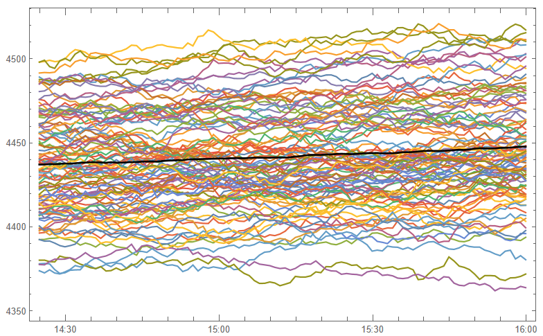
This indicates that the expected value of the SPX index at the close will be around 4450, which we could estimate directly from:

Where u is the estimated drift of the GBM process.

Similarly we can look at the projected terminal distribution of the index at 4pm to get a sense of the likely range of closing prices, which may assist a decision to open or close certain option (hedge) positions:

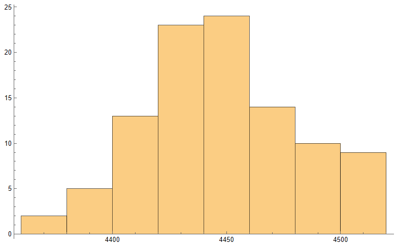
Of course, all this is predicated on the underlying process continuing on its current trajectory, with drift and standard deviation close to those seen in the process in the preceding time interval. But trends change, as do volatilities, which means that our forecasts may be inaccurate. Furthermore, the drift in asset processes tends to be dominated by volatility, especially at short time horizons.

So the best way to think of this is as a conditional expectation, i.e. “If the stock price continues on its current trajectory, then our expectation is that the closing price will be in the following range…”.

For more on MATH-TWS see:

MATH-TWS: Connecting Wolfram Mathematica to IB TWS

Transfer Learning

Building a deep learning neural network is a complicated and time-consuming task. For some problems it can be easier to re-purpose an existing deep learning model, making minor adjustments to a small number of layers to achieve desired architecture.

In his new book Introduction to Machine Learning, Etienne Bernard gives a nice example of the technique.

We begin with a dataset comprising images of two types of mushroom, with the aim of building a specialized image classifier.

Using a Neural Network for Feature Extraction

We start from the Wolfram ImageIdentify net, which is a 24-layer convolutional neural network trained on around 4000 image types.

net=NetModel[“Wolfram ImageIdentify Net V1”]

In its current form the net is too generalized for our task:

Mushroom

So instead of using the net in raw form, we use the first 22 layers as a feature extractor. This will preprocess each image to obtain features that are semantically richer than simple pixel values. We can then train a classifier on top of these new features, producing a logistic regression model:

c=Classify[dsTrain,FeatureExtractor->NetTake[net,22]]

The classifier can now distinguish between different types of mushrooms:

The classifier achieves around 88% accuracy on a test set constructed from a web image search:

dsTest = AssociationMap[
WebImageSearch[#, “Thumbnails”, 10] &, {“Morel”,
“Bolete”}] /. $Failed -> Nothing // Quiet;
ClassifierMeasurements[c, test, “Accuracy”,
ComputeUncertainty -> True]

0.88 +/- 0.09

This is much better than training directly on the underlying pixel values, which would result in an accuracy of around 44%, worse than random guessing.

Neural Network Transfer Learning

Moving on from Etienne’s feature extraction approach, we next try creating a new neural network by re-using the first 22 layers of the ImageIdentify network, adding two new layers (a LinearLayer and SoftmaxLayer) for mushroom classification:

changedNet=Drop[net,-2];
newNet=NetJoin[changedNet,NetChain[Association[“classifier”->LinearLayer[],”probabilities”->SoftmaxLayer[]],”Output”->NetDecoder[{“Class”,{“Bolete”,”Morel”}}]]]

We re-train the new network using the mushroom training dataset, holding the weights for the first 22 layers at their existing values (i.e. only training the last two, new layers):

trainedNet=NetTrain[newNet,Normal@dsTrain,LearningRateMultipliers->{“classifier”->1,_->0},BatchSize->16,TargetDevice->”GPU”]

Next, create a new test dataset and test the new neural network’s accuracy:

dsTest=AssociationMap[WebImageSearch[#,”Thumbnails”,10] &,{“Morel”,”Bolete”}] /. $Failed->Missing[] //Quiet;

The new net achieves 100% accuracy on the test dataset:

trainedNet[DeleteMissing@dsTest[“Bolete”]]

{“Bolete”, “Bolete”, “Bolete”, “Bolete”, “Bolete”, “Bolete”, \
“Bolete”, “Bolete”, “Bolete”}

trainedNet[DeleteMissing@dsTest[“Morel”]]

{“Morel”, “Morel”, “Morel”, “Morel”, “Morel”, “Morel”, “Morel”, \
“Morel”}