Quality Research vs. Poor Research
The stem paper for this post is:
Bao W, Yue J, Rao Y (2017) A deep learning framework for financial time series using
stacked autoencoders and long-short term memory. PLoS ONE 12(7): e0180944. https://doi.org/10.1371/journal.pone.0180944
The chief claim by the researchers is that 90% to 95% 1-day ahead forecast accuracy can be achieved for a selection of market indices, including the S&P500 and Dow Jones Industrial Average, using a deep learning network of stacked autoencoders and LSTM layers, acting on data transformed using the Haar Discrete Wavelet Transform. The raw data comprises daily data for the index, around a dozen standard technical indicators, the US dollar index and an interest rate series.
Before we go into any detail let’s just step back and look at the larger picture. We have:
- Unknown researchers
- A journal from outside the field of finance
- A paper replete with pretty colored images, but very skimpy detail on the methodology
- A claimed result that lies far beyond the bounds of credibility
There’s enough red flags here to start a stampede at Pamplona. Let’s go through them one by one:
- Everyone is unknown at some point in their career. But that’s precisely why you partner with a widely published author. It gives the reader confidence that the paper isn’t complete garbage.
- Not everyone gets to publish in the Journal of Finance. I get that. How many of us were regular readers of the Journal of Political Economy before Black and Scholes published their famous paper on option pricing in 1973? Nevertheless, a finance paper published in a medical journal does not inspire great confidence.
- Read almost any paper by a well known researcher and you will find copious detail on the methodology. These days, the paper is often accompanied by a Git repo (add 3 stars for this!). Academics producing quality research want readers to be able to replicate and validate their findings.
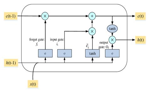
In this paper there are lots of generic, pretty colored graphics of deep learning networks, but no code repo and very little detail on the methodology. If you don’t want to publish details because the methodology is proprietary and potentially valuable, then do what I do: don’t publish at all. - One-day ahead forecasting accuracy of 53%-55% is good (52%-53% in HFT). 60% accuracy is outstanding. 90% – 95% is unbelievable. It’s a license to print money. So what we are being asked to believe is through a combination of data smoothing (which is all DWT is), dimensionality reduction (stacked autoencoders) and long-memory modeling, we can somehow improve forecasting accuracy over, say, a gradient boosted tree baseline, by something like 40%. It simply isn’t credible.
These simple considerations should be enough for any experienced quant to give the paper a wide berth.
Digging into the Methodology
- Discrete Wavelet Transform
So we start from a raw dataset with variables that closely match those described in the paper (see headers for details). Of course, I don’t know the parameter values they used for most of the technical indicators, but it possibly doesn’t matter all that much.
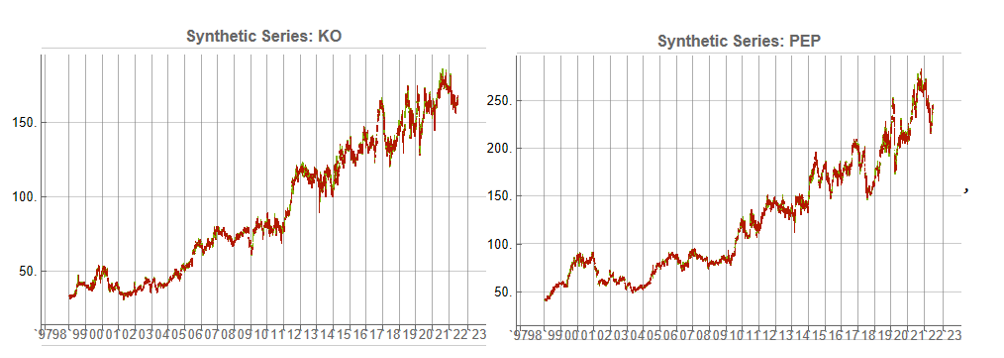
Note that I am applying DWT using the Haar wavelet twice: once to the original data and then again to the transformed data. This has the effect of filtering out higher frequency “noise” in the data, which is the object of the exercise. If follow this you will also see that the DWT actually adds noisy fluctuations to the US Dollar index and 13-Week TBill series. So these should be excluded from the de-noising process. You can see how the DWT denoising process removes some of the higher frequency fluctuations from the opening price, for instance:

2. Stacked Autoencoders
First up, we need to produce data for training, validation and testing. I am doing this for just the first batch of data. We would then move the window forward + 3 months, rinse and repeat.
Note that:
(1) The data is being standardized. If you don’t do this the outputs from the autoencoders is mostly just 1s and 0s. Same happens if you use Min/Max scaling.
(2) We use the mean and standard deviation from the training dataset to normalize the test dataset. This is a trap that too many researchers fall into – standardizing the test dataset using the mean and standard deviation of the test dataset is feeding forward information.
The Autoencoder stack uses a hidden layer of size 10 in each encoder. We strip the output layer from the first encoder and use the hidden layer as inputs to the second autoencoder, and so on:

3. Benchmark Model
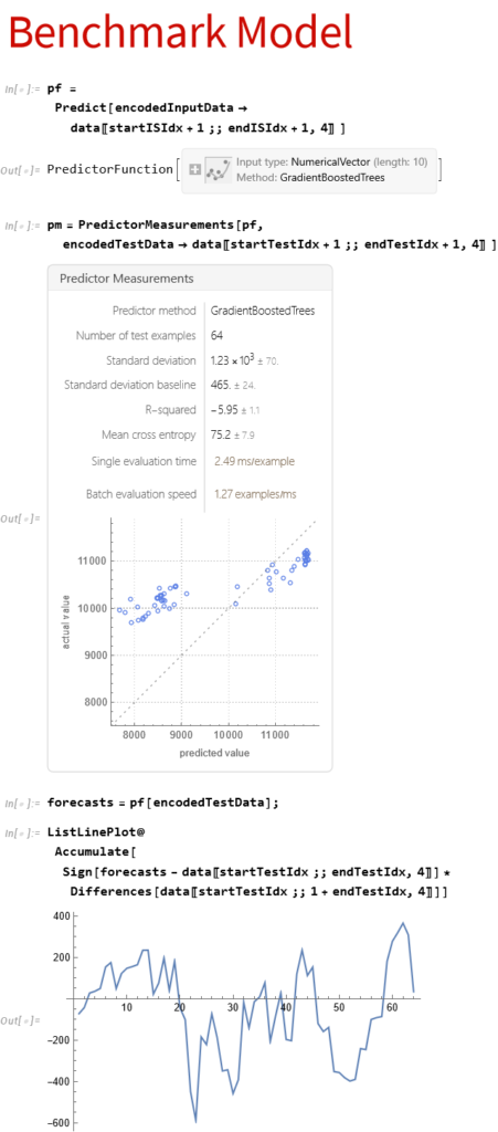
Before we plow on any further lets do a sanity check. We’ll use the Predict function to see if we’re able to get any promising-looking results. Here we are building a Gradient Boosted Trees predictor that maps the autoencoded training data to the corresponding closing prices of the index, one step ahead.
Next we use the predictor on the test dataset to produce 1-step-ahead forecasts for the closing price of the index.
Finally, we construct a trading model, as described in the paper, in which we go long or short the index depending on whether the forecast is above or below the current index level. The results do not look good (see below).
Now, admittedly, an argument can be made that a properly constructed LSTM model would outperform a simple gradient-boosted tree – but not by the amount that would be required to improve the prediction accuracy from around 50% to nearer 95%, the level claimed in the paper. At most I would expect to see a 1% to 5% improvement in forecast accuracy.
So what this suggests to me is that the researchers have got something wrong, by somehow allowing forward information to leak into the modeling process. The most likely culprits are:
- Applying DWT transforms to the entire dataset, instead of the training and test sets individually
- Standardzing the test dataset using the mean and standard deviation of the test dataset, instead of the training data set
A More Complete Attempt to Replicate the Research
There’s a much more complete attempt at replicating the research in this Git repo
As the repo author writes:
My attempts haven’t been succesful so far. Given the very limited comments regarding implementation in the article, it may be the case that I am missing something important, however the results seem too good to be true, so my assumption is that the authors have a bug in their own implementation. I would of course be happy to be proven wrong about this statement 😉
Conclusion
Over time, as one’s experience as a quant deepens, you learn to recognize the signs of shoddy research and save yourself the effort of trying to replicate it. It’s actually easier these days for researchers to fool themselves (and their readers) that they have uncovered something interesting, because of the facility with which complex algorithms can be deployed in an inappropriate way.
Postscript
This paper echos my concerns about the incorrect use of wavelets in a forecasting context:
The incorrect development of these wavelet-based forecasting models occurs during wavelet decomposition (the process of extracting high- and low-frequency information into different sub-time series known as wavelet and scaling coefficients, respectively) and as a result introduces error into the forecast model inputs. The source of this error is due to the boundary condition that is associated with wavelet decomposition (and the wavelet and scaling coefficients) and is linked to three main issues: 1) using ‘future data’ (i.e., data from the future that is not available); 2) inappropriately selecting decomposition levels and wavelet filters; and 3) not carefully partitioning calibration and validation data.
