Algorithmic Trading Archives - Page 4 of 4 - QUANTITATIVE RESEARCH AND TRADING

September 23, 2018September 23, 2018

High Frequency Trading with ADL – JonathanKinlay.com

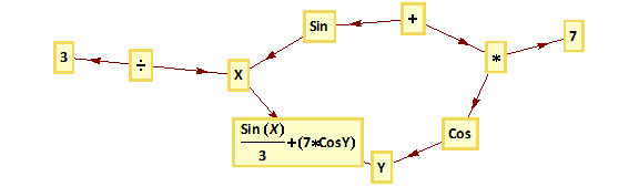
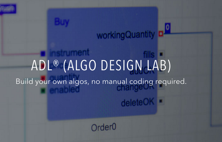
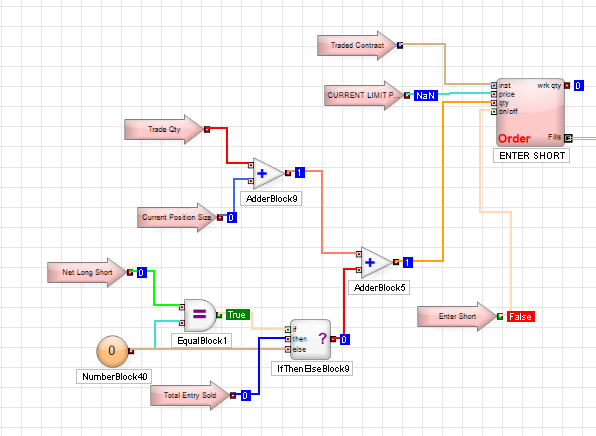
Trading Technologies’ ADL is a visual programming language designed specifically for trading strategy development that is integrated in the company’s flagship XTrader product. Despite the radically different programming philosophy, my experience of working with ADL has been delightfully easy and strategies that would typically take many months of coding in C++ have been up and running in a matter of days or weeks. An extract of one such strategy, a high frequency scalping trade in the E-Mini S&P 500 futures, is shown in the graphic above. The interface and visual language is so intuitive to a trading system developer that even someone who has never seen ADL before can quickly grasp at least some of what it happening in the code.

Strategy Development in Low vs. High-Level Languages
What are the benefits of using a high level language like ADL compared to programming languages like C++/C# or Java that are traditionally used for trading system development? The chief advantage is speed of development: I would say that ADL offers the potential up the development process by at least one order of magnitude. A complex trading system would otherwise take months or even years to code and test in C++ or Java, can be implemented successfully and put into production in a matter of weeks in ADL. In this regard, the advantage of speed of development is one shared by many high level languages, including, for example, Matlab, R and Mathematica. But in ADL’s case the advantage in terms of time to implementation is aided by the fact that, unlike generalist tools such as MatLab, etc, ADL is designed specifically for trading system development. The ADL development environment comes equipped with compiled pre-built blocks designed to accomplish many of the common tasks associated with any trading system such as acquiring market data and handling orders. Even complex spread trades can be developed extremely quickly due to the very comprehensive library of pre-built blocks.

Integrating Research and Development
One of the drawbacks of using a higher level language for building trading systems is that, being interpreted rather than compiled, they are simply too slow – one or more orders of magnitude, typically – to be suitable for high frequency trading. I will come on to discuss the execution speed issue a little later. For now, let me bring up a second major advantage of ADL relative to other high level languages, as I see it. One of the issues that plagues trading system development is the difficulty of communication between researchers, who understand financial markets well, but systems architecture and design rather less so, and developers, whose skill set lies in design and programming, but whose knowledge of markets can often be sketchy. These difficulties are heightened where researchers might be using a high level language and relying on developers to re-code their prototype system to get it into production. Developers typically (and understandably) demand a high degree of specificity about the requirement and if it’s not included in the spec it won’t be in the final deliverable. Unfortunately, developing a successful trading system is a highly non-linear process and a researcher will typically have to iterate around the core idea repeatedly until they find a combination of alpha signal and entry/exit logic that works. In other words, researchers need flexibility, whereas developers require specificity. ADL helps address this issue by providing a development environment that is at once highly flexible and at the same time powerful enough to meet the demands of high frequency trading in a production environment. It means that, in theory, researchers and developers can speak a common language and use a common tool throughout the R&D development cycle. This is likely to reduce the kind of misunderstanding between researchers and developers that commonly arise (often setting back the implementation schedule significantly when they do).

Latency
Of course, at least some of the theoretical benefit of using ADL depends on execution speed. The way the problem is typically addressed with systems developed in high level languages like Matlab or R is to recode the entire system in something like C++, or to recode some of the most critical elements and plug those back into the main Matlab program as dlls. The latter approach works, and preserves the most important benefits of working in both high and low level languages, but the resulting system is likely to be sub-optimal and can be difficult to maintain. The approach taken by Trading Technologies with ADL is very different. Firstly, the component blocks are written in C# and in compiled form should run about as fast as native code. Secondly, systems written in ADL can be deployed immediately on a co-located algo server that is plugged directly into the exchange, thereby reducing latency to an acceptable level. While this is unlikely to sufficient for an ultra-high frequency system operating on the sub-millisecond level, it will probably suffice for high frequency systems that operate at speeds above above a few millisecs, trading up to say, around 100 times a day.

Fill Rate and Toxic Flow
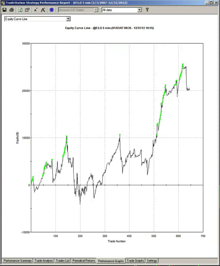
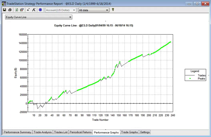
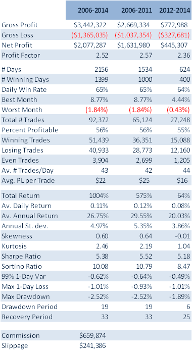
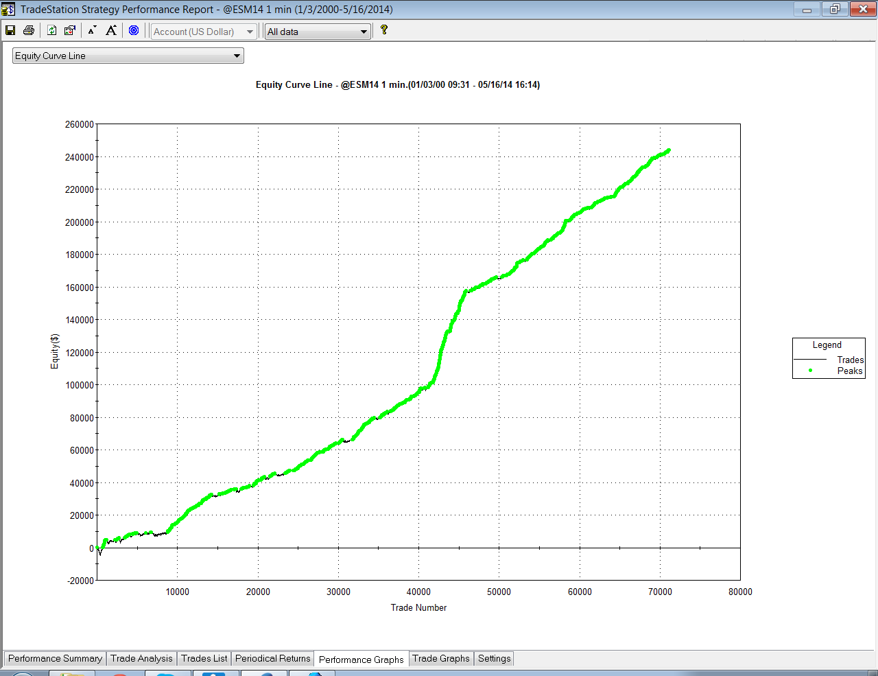
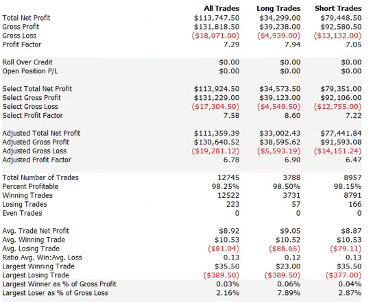
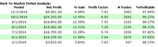
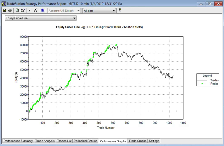
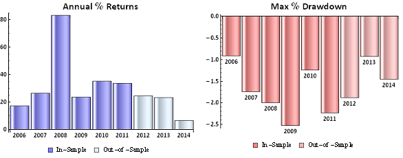
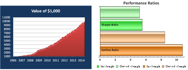
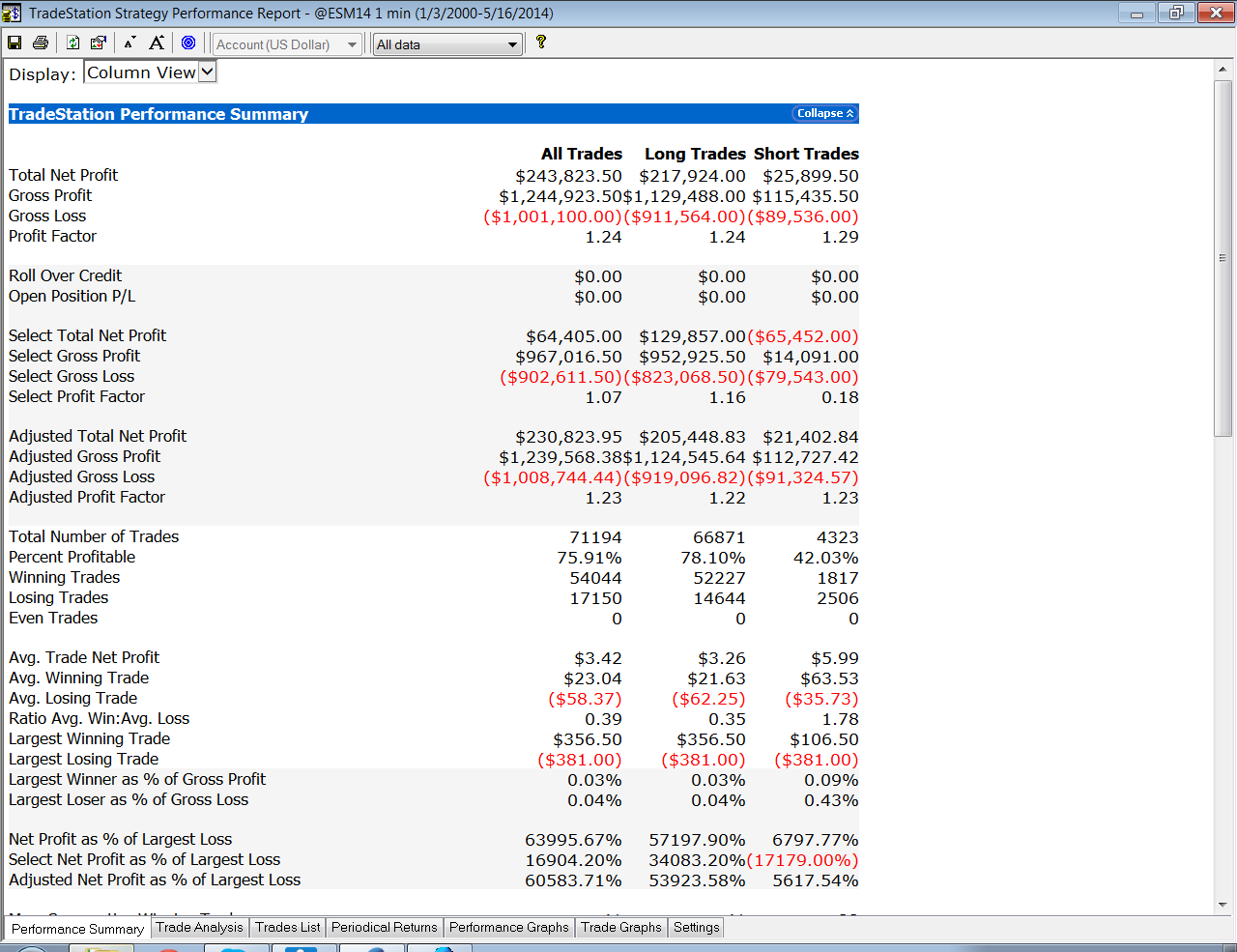
For those not familiar with the HFT territory, let me provide an example of why the issues of execution speed and latency are so important. Below is a simulated performance record for a HFT system in ES futures. The system is designed to enter and exit using limit orders and trades around 120 times a day, with over 98% profitability, if we assume a 100% fill rate. So far so good. But a 100% fill rate is clearly unrealistic. Let’s look at a pessimistic scenario: what if we got filled on orders only when the limit price was exceeded? 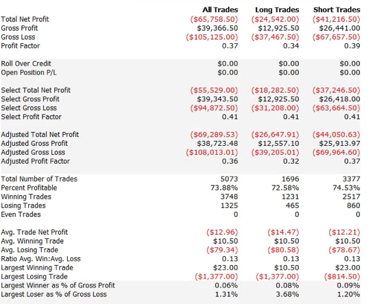(For those familiar with the jargon, we are assuming a high level of flow toxicity) The outcome is rather different: Neither scenario is particularly realistic, but the outcome is much more likely to be closer to the second scenario rather than the first if we our execution speed is slow, or if we are using a retail platform such as Interactive Brokers or Tradestation, with long latency wait times. The reason is simple: our orders will always arrive late and join the limit order book at the back of the queue. In most cases the orders ahead of ours will exhaust demand at the specified limit price and the market will trade away without filling our order. At other times the market will fill our order whenever there is a large flow against us (i.e. a surge of sell orders into our limit buy), i.e. when there is significant toxic flow. The proposition is that, using ADL and the its high-speed trading infrastructure, we can hope to avoid the latter outcome. While we will never come close to achieving a 100% fill rate, we may come close enough to offset the inevitable losses from toxic flow and produce a decent return. Whether ADL is capable of fulfilling that potential remains to be seen.

More on ADL
For more information on ADL go here.

September 11, 2018

How Not to Develop Trading Strategies – A Cautionary Tale

In his post on Multi-Market Techniques for Robust Trading Strategies (http://www.adaptrade.com/Newsletter/NL-MultiMarket.htm) Michael Bryant of Adaptrade discusses some interesting approaches to improving model robustness. One is to use data from several correlated assets to build the model, on the basis that if the algorithm works for several assets with differing price levels, that would tend to corroborate the system’s robustness. The second approach he advocates is to use data from the same asset series at different bars lengths. The example he uses @ES.D at 5, 7 and 9 minute bars. The argument in favor of this approach is the same as for the first, albeit in this case the underlying asset is the same.

I like Michael’s idea in principle, but I wanted to give you a sense of what can all too easily go wrong with GP modeling, even using techniques such as multi-time frame fitting and Monte Carlo simulation to improve robustness testing.

In the chart below I have extended the analysis back in time, beyond the 2011-2012 period that Michael used to build his original model. As you can see, most of the returns are generated in-sample, in the 2011-2012 period. As we look back over the period from 2007-2010, the results are distinctly unimpressive – the strategy basically trades sideways for four years.

How do Do It Right

In my view, there is only one, safe way to use GP to develop strategies. Firstly, you need to use a very long span of data – as much as possible, to fit your model. Only in this way can you ensure that the model has encountered enough variation in market conditions to stand a reasonable chance of being able to adapt to changing market conditions in future.

Secondly, you need to use two OOS period. The first OOS span of data, drawn from the start of the data series, is used in the normal way, to visually inspect the performance of the model. But the second span of OOS data, from more recent history, is NOT examined before the model is finalized. This is really important. Products like Adaptrade make it too easy for the system designer to “cheat”, by looking at the recent performance of his trading system “out of sample” and selecting models that do well in that period. But the very process of examining OOS performance introduces bias into the system. It would be like adding a line of code saying something like:

IF (model performance in OOS period > x) do the following….

I am quite sure if I posted a strategy with a line of code like that in it, it would immediately be shot down as being blatantly biased, and quite rightly so. But, if I look at the recent “OOS” performance and use it to select the model, I am effectively doing exactly the same thing.

That is why it is so important to have a second span of OOS data that it not only not used to build the model, but also is not used to assess performance, until after the final model selection is made. For that reason, the second OOS period is referred to as a “double blind” test.

That’s the procedure I followed to build my futures daytrading strategy: I used as much data as possible, dating from 2002. The first 20% of the each data set was used for normal OOS testing. But the second set of data, from Jan 2012 onwards, was my double-blind data set. Only when I saw that the system maintained performance in BOTH OOS periods was I reasonably confident of the system’s robustness.

This further explains why it is so challenging to develop higher frequency strategies using GP. Running even a very fast GP modeling system on a large span of high frequency data can take inordinate amounts of time.

The longest span of 5-min bar data that a GP system can handle would typically be around 5-7 years. This is probably not quite enough to build a truly robust system, although if you pick you time span carefully it might be (I generally like to use the 2006-2011 period, which has lots of market variation).

For 15 minute bar data, a well-designed GP system can usually handle all the available data you can throw at it – from 1999 in the case of the Emini, for instance.

Why I don’t Like Fitting Models over Short Time Spans

The risks of fitting models to data in short time spans are intuitively obvious. If you happen to pick a data set in which the market is in a strong uptrend, then your model is going to focus on that kind of market behavior. Subsequently, when the trend changes, the strategy will typically break down.
Monte Carlo simulation isn’t going to change much in this situation: sure, it will help a bit, perhaps, but since the resampled data is all drawn from the same original data set, in most cases the simulated paths will also show a strong uptrend – all that will be shown is that there is some doubt about the strength of the trend. But a completely different scenario, in which, say, the market drops by 10%, is unlikely to appear.

One possible answer to that problem, recommended by some system developers, is simply to rebuild the model when a breakdown is detected. While it’s true that a product like MSA can make detection easier, rebuilding the model is another question altogether. There is no guarantee that the kind of model that has worked hitherto can be re-tooled to work once again. In fact, there may be no viable trading system that can handle the new market dynamics.

Here is a case in point. We have a system that works well on 10 min bars in TF.D up until around May 2012, when MSA indicates a breakdown in strategy performance.

So now we try to fit a new model, along the pattern of the original model, taking account some of the new data. But it turns out to be just a Band-Aid – after a few more data points the strategy breaks down again, irretrievably.

This is typical of what often happens when you use GP to build a model using s short span of data. That’s why I prefer to use a long time span, even at lower frequency. The chances of being able to build a robust system that will adapt well to changing market conditions are much higher.

A Robust Emini Trading System

Here, for example is a GP system build on daily data in @ES.D from 1999 to 2011 (i.e. 2012 to 2014 is OOS).

September 9, 2018

Developing High Performing Trading Strategies with Genetic Programming

One of the frustrating aspects of research and development of trading systems is that there is never enough time to investigate all of the interesting trading ideas one would like to explore. In the early 1970’s, when a moving average crossover system was considered state of the art, it was relatively easy to develop profitable strategies using simple technical indicators. Indeed, research has shown that the profitability of simple trading rules persisted in foreign exchange and other markets for a period of decades. But, coincident with the advent of the PC in the late 1980’s, such simple strategies began to fail. The widespread availability of data, analytical tools and computing power has, arguably, contributed to the increased efficiency of financial markets and complicated the search for profitable trading ideas. We are now at a stage where is can take a team of 5-6 researchers/developers, using advanced research techniques and computing technologies, as long as 12-18 months, and hundreds of thousands of dollars, to develop a prototype strategy. And there is no guarantee that the end result will produce the required investment returns.

The lengthening lead times and rising cost and risk of strategy research has obliged trading firms to explore possibilities for accelerating the R&D process. One such approach is Genetic Programming.

Early Experiences with Genetic Programming
I first came across the GP approach to investment strategy in the late 1990s, when I began to work with Haftan Eckholdt, then head of neuroscience at Yeshiva University in New York. Haftan had proposed creating trading strategies by applying the kind of techniques widely used to analyze voluminous and highly complex data sets in genetic research. I was extremely skeptical of the idea and spent the next 18 months kicking the tires very hard indeed, of behalf of an interested investor. Although Haftan’s results seemed promising, I was fairly sure that they were the product of random chance and set about devising tests that would demonstrate that.

One of the challenges I devised was to create data sets in which real and synthetic stock series were mixed together and given to the system evaluate. To the human eye (or analyst’s spreadsheet), the synthetic series were indistinguishable from the real thing. But, in fact, I had “planted” some patterns within the processes of the synthetic stocks that made them perform differently from their real-life counterparts. Some of the patterns I created were quite simple, such as introducing a drift component. But other patterns were more nuanced, for example, using a fractal Brownian motion generator to induce long memory in the stock volatility process.

It was when I saw the system detect and exploit the patterns buried deep within the synthetic series to create sensible, profitable strategies that I began to pay attention. A short time thereafter Haftan and I joined forces to create what became the Proteom Fund.

That Proteom succeeded at all was a testament not only to Haftan’s ingenuity as a researcher, but also to his abilities as a programmer and technician. Processing such large volumes of data was a tremendous challenge at that time and required a cluster of 50 cpu’s networked together and maintained with a fair amount of patch cable and glue. We housed the cluster in a rat-infested warehouse in Brooklyn that had a very pleasant view of Manhattan, but no a/c. The heat thrown off from the cluster was immense, and when combined with very loud rap music blasted through the walls by the neighboring music studios, the effect was debilitating. As you might imagine, meetings with investors were a highly unpredictable experience. Fortunately, Haftan’s intellect was matched by his immense reserves of fortitude and patience and we were able to attract investments from several leading institutional investors.

The Genetic Programming Approach to Building Trading Models

Genetic programming is an evolutionary-based algorithmic methodology which can be used in a very general way to identify patterns or rules within data structures. The GP system is given a set of instructions (typically simple operators like addition and subtraction), some data observations and a fitness function to assess how well the system is able to combine the functions and data to achieve a specified goal.

In the trading strategy context the data observations might include not only price data, but also price volatility, moving averages and a variety of other technical indicators. The fitness function could be something as simple as net profit, but might represent alternative measures of profitability or risk, with factors such as PL per trade, win rate, or maximum drawdown. In order to reduce the danger of over-fitting, it is customary to limit the types of functions that the system can use to simple operators (+,-,/,*), exponents, and trig functions. The length of the program might also be constrained in terms of the maximum permitted lines of code.

We can represent what is going on using a tree graph:

In this example the GP system is combining several simple operators with the Sin and Cos trig functions to create a signal comprising an expression in two variables, X and Y, which may be, for example, stock prices, moving averages, or technical indicators of momentum or mean reversion.
The “evolutionary” aspect of the GP process derives from the idea that an existing signal or model can be mutated by replacing nodes in a branch of a tree, or even an entire branch by another. System performance is re-evaluated using the fitness function and the most profitable mutations are retained for further generation.
The resulting models are often highly non-linear and can be very general in form.

A GP Daytrading Strategy
The last fifteen years has seen tremendous advances in the field of genetic programming, in terms of the theory as well as practice. Using a single hyper-threaded CPU, it is now possible for a GP system to generate signals at a far faster rate than was possible on Proteom’s cluster of 50 networked CPUs. A researcher can develop and evaluate tens of millions of possible trading algorithms with the space of a few hours. Implementing a thoroughly researched and tested strategy is now feasible in a matter of weeks. There can be no doubt of GP’s potential to produce dramatic reductions in R&D lead times and costs. But does it work?

To address that question I have summarized below the performance results from a GP-developed daytrading system that trades nine different futures markets: Crude Oil (CL), Euro (EC), E-Mini (ES), Gold (GC), Heating Oil (HO), Coffee (KC), Natural gas (NG), Ten Year Notes (TY) and Bonds (US). The system trades a single contract in each market individually, going long and short several times a day. Only the most liquid period in each market is traded, which typically coincides with the open-outcry session, with any open positions being exited at the end of the session using market orders. With the exception of the NG and HO markets, which are entered using stop orders, all of the markets are entered and exited using standard limit orders, at prices determined by the system

The system was constructed using 15-minute bar data from Jan 2006 to Dec 2011 and tested out-of-sample of data from Jan 2012 to May 2014. The in-sample span of data was chosen to cover periods of extreme market stress, as well as less volatile market conditions. A lengthy out-of-sample period, almost half the span of the in-sample period, was chosen in order to evaluate the robustness of the system.
Out-of-sample testing was “double-blind”, meaning that the data was not used in the construction of the models, nor was out-of-sample performance evaluated by the system before any model was selected.

Performance results are net of trading commissions of $6 per round turn and, in the case of HO and NG, additional slippage of 2 ticks per round turn.

(click on the table for a higher definition view)

The most striking feature of the strategy is the high rate of risk-adjusted returns, as measured by the Sharpe ratio, which exceeds 5 in both in-sample and out-of-sample periods. This consistency is a reflection of the fact that, while net returns fall from an annual average of over 29% in sample to around 20% in the period from 2012, so, too, does the strategy volatility decline from 5.35% to 3.86% in the respective periods. The reduction in risk in the out-of-sample period is also reflected in lower Value-at-Risk and Drawdown levels.

A decline in the average PL per trade from $25 to $16 in offset to some degree by a slight increase in the rate of trading, from 42 to 44 trades per day, on average, while daily win rate and percentage profitable trades remain consistent at around 65% and 56%, respectively.

Overall, the system appears to be not only highly profitable, but also extremely robust. This is impressive, given that the models were not updated with data after 2011, remaining static over a period almost half as long as the span of data used in their construction. It is reasonable to expect that out-of-sample performance might be improved by allowing the models to be updated with more recent data.

Benefits and Risks of the GP Approach to Trading System Development
The potential benefits of the GP approach to trading system development include speed of development, flexibility of design, generality of application across markets and rapid testing and deployment.

What about the downside? The most obvious concern is the risk of over-fitting. By allowing the system to develop and test millions of models, there is a distinct risk that the resulting systems may be too closely conditioned on the in-sample data, and will fail to maintain performance when faced with new market conditions. That is why, of course, we retain a substantial span of out-of-sample data, in order to evaluate the robustness of the trading system. Even so, given the enormous number of models evaluated, there remains a significant risk of over-fitting.

Another drawback is that, due to the nature of the modelling process, it can be very difficult to understand, or explain to potential investors, the “market hypothesis” underpinning any specific model. “We tested it and it works” is not a particularly enlightening explanation for investors, who are accustomed to being presented with a more articulate theoretical framework, or investment thesis. Not being able to explain precisely how a system makes money is troubling enough in good times; but in bad times, during an extended drawdown, investors are likely to become agitated very quickly indeed if no explanation is forthcoming. Unfortunately, evaluating the question of whether a period of poor performance is temporary, or the result of a breakdown in the model, can be a complicated process.

Finally, in comparison with other modeling techniques, GP models suffer from an inability to easily update the model parameters based on new data as it become available. Typically, as GP model will be to rebuilt from scratch, often producing very different results each time.

Conclusion
Despite the many limitations of the GP approach, the advantages in terms of the speed and cost of researching and developing original trading signals and strategies have become increasingly compelling.

Given the several well-documented successes of the GP approach in fields as diverse as genetics and physics, I think an appropriate position to take with respect to applications within financial market research would be one of cautious optimism.

September 8, 2018

A Scalping Strategy in E-Mini Futures

This is a follow up post to my post on the Mathematics of Scalping. To illustrate the scalping methodology, I coded up a simple strategy based on the techniques described in the post.

The strategy trades a single @ES contract on 1-minute bars. The attached ELD file contains the Easylanguage code for ES scalping strategy, which can be run in Tradestation or Multicharts.

This strategy makes no attempt to forecast market direction and doesn’t consider market trends at all. It simply looks at the current levels of volatility and takes a long volatility position or a short volatility position depending on whether volatility is above or below some threshold parameters.

By long volatility I mean a position where we buy or sell the market and set a loose Profit Target and a tight Stop Loss. By short volatility I mean a position where we buy or sell the market and set a tight Profit Target and loose Stop Loss. This is exactly the methodology I described earlier in the post. The parameters I ended up using are as follows:

Long Volatility: Profit Target = 8 ticks, Stop Loss = 2 ticks
Short Volatility: Profit Target = 2 ticks, Stop Loss = 30 ticks

I have made no attempt to optimize these parameters settings, which can easily be done in Tradestation or Multicharts.

What do we mean by volatility being above our threshold level? I use a very simple metric: I take the TrueRange for the current bar and add 50% of the increase or decrease in TrueRange over the last two bars. That’s my crude volatility “forecast”.

The final point to explain is this: let’s suppose our volatility forecast is above our threshold level, so we know we want to be long volatility. Ok, but do we buy or sell the ES? One approach ia to try to gauge the direction of the market by estimating the trend. Not a bad idea, by any means, although I have argued that volatility drowns out any trend signal at short time frames (like 1 minute, for example). So I prefer an approach that makes no assumptions about market direction.

In this approach what we do is divide volatility into upsideVolatility and downsideVolatility. upsideVolatility uses the TrueRange for bars where Close > Close[1]. downsideVolatility is calculated only for bars where Close < Close[1]. This kind of methodology, where you calculate volatility based on the sign of the returns, is well known and is used in performance measures like the Sortino ratio. This is like the Sharpe ratio, except that you calculate the standard deviation of returns using only days in which the market was down. When it’s calculated this way, standard deviation is known as the (square root of the) semi-variance.

Anyway, back to our strategy. So we calculate the upside and downside volatilities and test them against our upper and lower volatility thresholds.

The decision tree looks like this:

LONG VOLATILITY
If upsideVolatilityForecast > upperVolThrehold, buy at the market with wide PT and tight ST (long market, long volatility)
If downsideVolatilityForecast > upperVolThrehold, sell at the market with wide PT and tight ST (short market, long volatility)

SHORT VOLATILITY
If upsideVolatilityForecast < lowerVolThrehold, sell at the Ask on a limit with tight PT and wide ST (short market, short volatility)
If downsideVolatilityForecast < lowerVolThrehold, buy at the Bid on a limit with tight PT and wide ST (long market, short volatility)

NOTE THE FOLLOWING CAVEATS. DO NOT TRY TO TRADE THIS STRATEGY LIVE (but use it as a basis for a tradable strategy)

1. The strategy makes the usual TS assumption about fill rates, which is unrealistic, especially at short intervals like 1-minute.
2. The strategy allows fees and commissions of $3 per contract, or $6 per round turn. Your trading costs may be higher than this.
3. Tradestation is unable to perform analysis at the tick level for a period as long at the one used here (2000 to 2014). A tick by tick analysis would likely show very different results (better or worse).
4. The strategy is extremely lop-sided: the great majority of the profits are made on the long side and the Win Rates and Profit Factors are very different for long trades vs short trades. I suspect this would change with a tick by tick analysis. But it also may be necessary to add more parameters so that long trades are treated differently from short trades.
5. No attempt has been made to optimize the parameters.
6 This is a daytading strategy that will exit the market on close.

So with all that said here are the results.

As you can see, the strategy produces a smooth, upward sloping equity curve, the slope of which increases markedly during the period of high market volatility in 2008.
Net profits after commissions for a single ES contract amount to $243,000 ($3.42 per contract) with a win rate of 76% and Profit Factor of 1.24.

This basic implementation would obviously require improvement in several areas, not least of which would be to address the imbalance in strategy profitability on the short vs long side, where most of the profits are generated.