Optimal Mean-Reversion Strategies

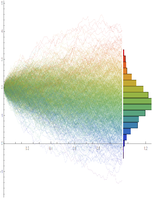
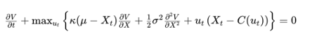
Consider a financial asset whose price, Xt​, follows a mean-reverting stochastic process. A common model for mean reversion is the Ornstein-Uhlenbeck (OU) process, defined by the stochastic differential equation (SDE):

The trader aims to maximize the expected cumulative profit from trading this asset over a finite horizon, subject to transaction costs. The trader’s control is the rate of buying or selling the asset, denoted by ut​, at time t.

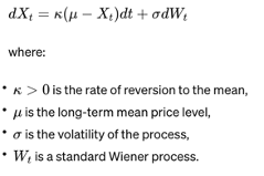
To find the optimal trading strategy, we frame this as a stochastic control problem. The value function,V(t,Xt​), represents the maximum expected profit from time t to the end of the trading horizon, given the current price level Xt​. The HJB equation for this problem is:

where C(ut​) represents the cost of trading, which can depend on the rate of trading ut​. The term ut​(Xt​−C(ut​)) captures the profit from trading, adjusted for transaction costs.

Boundary and Terminal Conditions: Specify terminal conditions for V(T,XT​), where T is the end of the trading horizon, and boundary conditions for V(t,Xt​) based on the problem setup.

Solve the HJB Equation: The solution involves finding the function V(t,Xt​) and the control policy ut∗​ that maximizes the HJB equation. This typically requires numerical methods, especially for complex cost functions or when closed-form solutions are not feasible.

Interpret the Optimal Policy: The optimal control ut∗​ derived from solving the HJB equation indicates the optimal rate of trading (buying or selling) at any time t and price level Xt​, considering the mean-reverting nature of the price and the impact of transaction costs.

No-Trade Zones: The presence of transaction costs often leads to the creation of no-trade zones in the optimal policy, where the expected benefit from trading does not outweigh the costs.

Mean-Reversion Exploitation: The optimal strategy exploits mean reversion by adjusting the trading rate based on the deviation of the current price from the mean level, μ.

The Lipton & Lopez de Marcos Paper

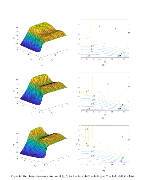
“A Closed-form Solution for Optimal Mean-reverting Trading Strategies” contributes significantly to the literature on optimal trading strategies for mean-reverting instruments. The paper focuses on deriving optimal trading strategies that maximize the Sharpe Ratio by solving the Hamilton-Jacobi-Bellman equation associated with the problem. It outlines a method that relies on solving a Fredholm integral equation to determine the optimal trading levels, taking into account transaction costs.

The paper begins by discussing the relevance of mean-reverting trading strategies across various markets, particularly emphasizing the energy market’s suitability for such strategies. It acknowledges the practical challenges and limitations of previous analytical results, mainly asymptotic and applicable to perpetual trading strategies, and highlights the novelty of addressing finite maturity strategies.

A key contribution of the paper is the development of an explicit formula for the Sharpe ratio in terms of stop-loss and take-profit levels, which allows traders to deploy tactical execution algorithms for optimal strategy performance under different market regimes. The methodology involves calibrating the Ornstein-Uhlenbeck process to market prices and optimizing the Sharpe ratio with respect to the defined levels. The authors present numerical results that illustrate the Sharpe ratio as a function of these levels for various parameters and discuss the implications of their findings for liquidity providers and statistical arbitrage traders.

The paper also reviews traditional approaches to similar problems, including the use of renewal theory and linear transaction costs, and compares these with its analytical framework. It concludes that its method provides a valuable tool for liquidity providers and traders to optimally execute their strategies, with practical applications beyond theoretical interest.

The authors use the path integral method to understand the behavior of their solutions, providing an alternative treatment to linear transaction costs that results in a determination of critical boundaries for trading. This approach is distinct in its use of direct solving methods for the Fredholm equation and adjusting the trading thresholds through a numerical method until a matching condition is met.

This research not only advances the understanding of optimal trading rules for mean-reverting strategies but also offers practical guidance for traders and liquidity providers in implementing these strategies effectively.

Intraday Stock Index Forecasting

In a previous post I discussed modelling stock prices processes as Geometric brownian Motion processes:

Understanding Stock Price Range Forecasts

To recap briefly, we assume a process of the form:

Where S0 is the initial stock price at time t = 0.

The mean of such a process is:

and standard deviation:

In the post I showed how to estimate such a process with daily stock prices, using these to provide a forecast range of prices over a one-month horizon. This is potentially useful, for example, in choosing which strikes to select in an option hedge.

Of course, there is nothing to prevent you from using the same technique over different timescales. Here I use the MATH-TWS package to connect Mathematica to the IB TWS platform via the C++ api, to extract intraday prices for the S&P 500 Index at 1-minute intervals. These are used to estimate a short-term GBM process, which provides forecasts of the mean and variance of the index at the 4 PM close.

We capture the data using:

then create a time series of the intraday prices and plot them:

If we want something a little fancier we can create a trading chart, including technical indicators of our choice, for instance:

The charts can be updated in real time from IB, using MATHTWS.

From there we estimate a GBM process using 1-minute close prices:

and then simulate a number of price paths towards the 4 PM close (the mean price path is shown in black):

This indicates that the expected value of the SPX index at the close will be around 4450, which we could estimate directly from:

Where u is the estimated drift of the GBM process.

Similarly we can look at the projected terminal distribution of the index at 4pm to get a sense of the likely range of closing prices, which may assist a decision to open or close certain option (hedge) positions:

Of course, all this is predicated on the underlying process continuing on its current trajectory, with drift and standard deviation close to those seen in the process in the preceding time interval. But trends change, as do volatilities, which means that our forecasts may be inaccurate. Furthermore, the drift in asset processes tends to be dominated by volatility, especially at short time horizons.

So the best way to think of this is as a conditional expectation, i.e. “If the stock price continues on its current trajectory, then our expectation is that the closing price will be in the following range…”.

For more on MATH-TWS see:

MATH-TWS: Connecting Wolfram Mathematica to IB TWS

Understanding Stock Price Range Forecasts

Stock Price Range Forecasts

Range forecasts are produced by estimating the parameters of a Geometric Brownian Motion process from historical data and using the model to project a large number of sample paths for the stock price over the coming month and year.

For example, this is a range forecast for Netflix, Inc. (NFLX) as at 7/27/2018 when the price of the stock stood at $355.21:

$NFLX

As you can see, the great majority of the simulated price paths trend upwards.  This is typical for most stocks on account of their upward drift, a tendency to move higher over time.  The statistical table below the chart tells you that in 50% of cases the ending stock price 1 month from the date of forecast was in the range $352.15 to $402.49. Similarly, around 50% of the time the price of the stock in one year’s time were found to be in the range $565.01 to $896.69.  Notice that the end points of the one-year range far exceed the end points of the one-month range forecast – again this is a feature of the upward drift in stocks.

If you want much greater certainty about the outcome, you should look at the 95% ranges.  So, for NFLX, the one month 95% range was projected to be $310.06 to $457.13.  Here, only 1 in 20 of the simulated price paths produced one month forecasts that were higher than $457.13, or lower than $310.06.

Notice that the spread of the one month and one year 95% ranges is much larger than of the corresponding 50% ranges.  This demonstrates the fundamental tradeoff between “accuracy” (the spread of the range) and “certainty”, (the probability of the outcome being with the projected range).  If you want greater certainty of the outcome, you have to allow for a broader span of possibilities, i.e. a wider range.

SSALGOTRADING AD

Uses of Range Forecasts

Most stock analysts tend to produce single price “targets”, rather than a range – these are known as “point forecasts” by econometricians.  So what’s the thinking behind range forecasts?

Range forecasts are arguably more useful than simple point forecasts.  Point forecasts make no guarantee as to the likelihood of the projected price – the only thing we know for sure about such forecasts is that they will be wrong!  Is the forecast target price optimistic or pessimistic?  We have no way to tell.

With range forecasts the situation is very different.  We can talk about the likelihood of a stock being within a specified range at a certain point in time.  If we want to provide a pessimistic forecast for the price in NFLX in one month’s time, for example, we could quote the value $352.15, the lower end of the 50% range forecast.  If we wanted to provide a very pessimistic forecast, one that is very likely to be exceeded, we could quote the bottom of the 95% range: $310.06.

The range also tells us about the future growth prospects for the firm.  So, for example, with NFLX, based on past performance, it is highly likely that the stock price will grow at a rate of more than 2.4% and, optimistically, might increase by almost 3x in the coming year (see the growth rates calculated for the 95% range values).

One specific use of range forecasts is in options trading.  If a trader is bullish on NFLX, instead of buying the stock, he might instead choose to sell one-month put options with a strike price below $352 (the lower end of the 50% one-month range).  If the trader wanted to be more conservative, he might look for put options struck at around $310, the bottom of the 95% range.  A more complex strategy might be to buy calls struck near the top of the 50% range, and sell more calls struck near the top of the 95% range (the theory being that the stock is quite likely to exceed the top of the 50% one-month range, but much less likely to reach the high end of the 95% range).

Limitations of Range Forecasts

Range forecasts are produced by using historical data to estimate the parameters of a particular type of mathematical model, known as a Geometric Brownian Motion process.  For those who are interested in the mechanics of how the forecasts are produced, I have summarized the relevant background theory below.

While there are grounds for challenging the use of such models in this context, it has to be acknowledged that the GBM process is one of the most successful mathematical models in finance today.  The problem lies not so much in the model, as in one of the key assumptions underpinning the approach:  specifically, that the characteristics of the stock process will remain as they are today (and as they have been in the historical past).  This assumption is manifestly untenable when applied to many stocks:  a company that was a high-growth $100M start-up is unlikely to demonstrate the same  rate of growth ten years later, as a $10Bn enterprise.  A company like Amazon that started out as an online book seller has fundamentally different characteristics today, as an online retail empire.  In such cases, forecasts about the future stock price – whether point or range forecasts – based on outdated historical informations are likely to be wrong, sometimes wildly so.

Having said that, there are a great many companies that have evolved to a point of relative stability over a period of perhaps several decades: for example, a company like Caterpillar Inc. (CAT).  In such cases the parameters of the GBM process underpinning the stock price are unlikely to fluctuate widely in the short term, so range forecasts are consequently more likely to be useful.

Another factor to consider are quarterly earnings reports, which can influence stock prices considerably in the short term, and corporate actions (mergers, takeovers, etc) that can change the long term characteristics of a firm and its stock price process in a fundamental way.  In these situations any forecast methodology is likely to unreliable, at least for a while, until the event has passed.  It’s best to avoid taking positions based on projections from historical data at times like this.

Review of Background Theory


GBM1

GBM2 GBM3 GBM4 GBM5

Modeling Asset Processes

Introduction

Over the last twenty five years significant advances have been made in the theory of asset processes and there now exist a variety of mathematical models, many of them computationally tractable, that provide a reasonable representation of their defining characteristics.

SSALGOTRADING AD

While the Geometric Brownian Motion model remains a staple of stochastic calculus theory, it is no longer the only game in town.  Other models, many more sophisticated, have been developed to address the shortcomings in the original.  There now exist models that provide a good explanation of some of the key characteristics of asset processes that lie beyond the scope of models couched in a simple Gaussian framework. Features such as mean reversion, long memory, stochastic volatility,  jumps and heavy tails are now readily handled by these more advanced tools.

In this post I review a critical selection of asset process models that belong in every financial engineer’s toolbox, point out their key features and limitations and give examples of some of their applications.


Modeling Asset Processes