Machine Learning Archives - Page 3 of 3 - QUANTITATIVE RESEARCH AND TRADING

August 20, 2019

The Swan of Deadwood

Spending 12-14 hours a day managing investors’ money doesn’t leave me a whole lot of time to sit around watching TV. And since I have probably less than 10% of the ad-tolerance of a typical American audience member, I inevitably turn to TiVo, Netflix, or similar, to watch a commercial-free show. Which means that I am inevitably several years behind the cognoscenti of the au-courant. This has its pluses: I avoid a lot of drivel that way.

So it was that I recently tuned in to watch Deadwood, a masterpiece of modern drama written by the talented David Milch, of NYPD Blue fame. The setting of the show is unpromising: a mud-caked camp in South Dakota around the turn of the 19th century that appears to portend yet another formulaic Western featuring liquor, guns, gals and gold and not much else. The first episode appeared at first to confirm my lowest expectations. I struggled through the second. But by the third I was hooked.

What makes Deadwood such a triumph are its finely crafted plots and intricate sub-plots; the many varied and often complex characters, superbly played by Ian McShane (with outstanding performances by Brad Dourif, Powers Boothe, amongst an abundance of others, no less gifted); and, of course, the dialogue.

Yes, the dialogue: hardly the crowning glory of the typical Hollywood Western. And here, to make matters worse, almost every sentence uttered by many of the characters is replete with such shocking profanity that one is eventually numbed into accepting it as normal. But once you get past that, something strange and rather wonderful overtakes you: a sense of being carried along on a river of creative wordsmith-ing that at times eddies, bubbles, plunges and roars its way through scenes that are as comedic, dramatic and action-packed as any I have seen on film. For those who have yet to enjoy the experience, I offer one small morsel:

https://www.youtube.com/watch?v=RdJ4TQ3TnNo

Milch as Shakespeare?

Around the start of Series 2 a rather strange idea occurred to me that, try as I might, I was increasingly unable to suppress as the show progressed: that the writing – some of it at least – was almost Shakespearian in its ingenuity and, at times, lyrical complexity.

Convinced that I had taken leave of my senses I turned to Google and discovered, to my surprise, that there is a whole cottage industry of Deadwood fans who had made the same connection. There is even – if you can imagine it – an online quiz that tests if you are able to identify the source of a number of quotes that might come from the show, or one of the Bard’s many plays. I kid you not:

Intrigued, I took the test and scored around 85%. Not too bad for a science graduate, although I expect most English majors would top 90%-95%. That gave me an idea: could one develop a machine learning algorithm to do the job?

Here’s how it went.

Milch or Shakespeare? – A Machine Learning Classification Algorithm

We start by downloading the text of a representative selection of Shakespeare’s plays, avoiding several of the better-known works from which many of the quotations derive:

For testing purposes, let’s download a sample of classic works by other authors:

Let’s build an initial test classifier, as follows:

It seems to work ok:

So far so good. Let’s import the script for Deadwood series 1-3:

DeadWood = Import[“……../Dropbox/Documents/Deadwood-Seasons-1-3-script.txt”];

Next, let’s import the quotations used in the online test:

etc

We need to remove the relevant quotes from the Deadwood script file used to train the classifier, of course (otherwise it’s cheating!). We will strip an additional 200 characters before the start of each quotation, and 500 characters after each quotation, just for good measure:

and so on….

Now we are ready to build our classifier:

And we can obtain some information about the classifier, as follows:

Let’s see how it performs:

Or, if you prefer tabular form:

The machine learning model scored a total of 19 correct answers out of 23, or 82%.

Fooling the Machine

Let’s take a look as some of the questions the algorithm got wrong.

Quotation no. 13 is challenging, as it comes from Pericles, one of Shakespeare’s lesser-know plays and the idiom appears entirely modern. The classifier assigns an 87% probability of Milch being the author (I got it wrong too).

On Quotation no. 15 the algorithm was just as mistaken, but in the other direction (I got this one right, but only because I recalled the monologue from the episode):

Quotation no.16 strikes me as entirely Shakespearian in form and expression and the classifier thought so too, favoring the Bard by 86% to only 14% for Milch:

Quotation no. 19 had the algorithm fooled completely. It’s a perfect illustration of a typical kind of circumlocution favored by Shakespeare that is imitated so well by Milch’s Deadwood characters:

Conclusion

The model clearly picked up distinguishing characteristics of the two authors’ writings that enabled it to correctly classify 82% of the quotations, quite a high percentage and much better than we would expect to do by tossing a coin, for example. It’s a respectable performance, but I might have hoped for greater accuracy from the model, which scored about the same as I did.

I guess those who see parallels in the writing of William Shakespeare and David Milch may be onto something.

Postscript

The Hollywood Reporter recently published a story entitled

“How the $100 Million ‘NYPD Blue’ Creator Gambled Away His Fortune”.

It’s a fascinating account of the trials and tribulations of this great author, one worthy of Deadwood itself.

A silver lining to this tragic tale, perhaps, is that Milch’s difficulties may prompt him into writing the much-desired Series 4.

One can hope.

January 22, 2019

Identifying Drivers of Trading Strategy Performance

Building a winning strategy, like the one in the e-Mini S&P500 futures described here is only half the challenge: it remains for the strategy architect to gain an understanding of the sources of strategy alpha, and risk. This means identifying the factors that drive strategy performance and, ideally, building a model so that their relative importance can be evaluated. A more advanced step is the construction of a meta-model that will predict strategy performance and provided recommendations as to whether the strategy should be traded over the upcoming period.

Strategy Performance – Case Study

Let’s take a look at how this works in practice. Our case study makes use of the following daytrading strategy in e-Mini futures.

The overall performance of the strategy is quite good. Average monthly PNL over the period from April to Oct 2015 is almost $8,000 per contract, after fees, with a standard deviation of only $5,500. That equates to an annual Sharpe Ratio in the region of 5.0. On a decent execution platform the strategy should scale to around 10-15 contracts, with an annual PNL of around $1.0 to $1.5 million.

Looking into the performance more closely we find that the win rate (56%) and profit factor (1.43) are typical for a profitable strategy of medium frequency, trading around 20 times per session (in this case from 9:30AM to 4PM EST).

Another attractive feature of the strategy risk profile is the Max Adverse Execution, the drawdown experienced in individual trades (rather than the realized drawdown). In the chart below we see that the MAE increases steadily, without major outliers, to a maximum of only around $1,000 per contract.

One concern is that the average trade PL is rather small – $20, just over 1.5 ticks. Strategies that enter and exit with limit orders and have small average trade are generally highly dependent on the fill rate – i.e. the proportion of limit orders that are filled. If the fill rate is too low, the strategy will be left with too many missed trades on entry or exit, or both. This is likely to damage strategy performance, perhaps to a significant degree – see, for example my post on High Frequency Trading Strategies.

The fill rate is dependent on the number of limit orders posted at the extreme high or low of the bar, known as the extreme hit rate. In this case the strategy has been designed specifically to operate at an extreme hit rate of only around 10%, which means that, on average, only around one trade in ten occurs at the high or low of the bar. Consequently, the strategy is not highly fill-rate dependent and should execute satisfactorily even on a retail platform like Tradestation or Interactive Brokers.

Drivers of Strategy Performance

So far so good. But before we put the strategy into production, let’s try to understand some of the key factors that determine its performance. Hopefully that way we will be better placed to judge how profitable the strategy is likely to be as market conditions evolve.

In fact, we have already identified one potential key performance driver: the extreme hit rate (required fill rate) and determined that it is not a major concern in this case. However, in cases where the extreme hit rate rises to perhaps 20%, or more, the fill ratio is likely to become a major factor in determining the success of the strategy. It would be highly inadvisable to attempt implementation of such a strategy on a retail platform.

What other factors might affect strategy performance? The correct approach here is to apply the scientific method: develop some theories about the drivers of performance and see if we can find evidence to support them.

For this case study we might conjecture that, since the strategy enters and exits using limit orders, it should exhibit characteristics of a mean reversion strategy, which will tend to do better when the market moves sideways and rather worse in a strongly trending market.

Another hypothesis is that, in common with most day-trading and high frequency strategies, this strategy will produce better results during periods of higher market volatility. Empirically, HFT firms have always produced higher profits during volatile market conditions – 2008 was a banner year for many of them, for example. In broad terms, times when the market is whipsawing around create additional opportunities for strategies that seek to exploit temporary mis-pricings. We shall attempt to qualify this general understanding shortly. For now let’s try to gather some evidence that might support the hypotheses we have formulated.

I am going to take a very simple approach to this, using linear regression analysis. It’s possible to do much more sophisticated analysis using nonlinear methods, including machine learning techniques. In our regression model the dependent variable will be the daily strategy returns. In the first iteration, let’s use measures of market returns, trading volume and market volatility as the independent variables.

The first surprise is the size of the (adjusted) R Square – at 28%, this far exceeds the typical 5% to 10% level achieved in most such regression models, when applied to trading systems. In other words, this model does a very good job of account for a large proportion of the variation in strategy returns.

Note that the returns in the underlying S&P50o index play no part (the coefficient is not statistically significant). We might expect this: ours is is a trading strategy that is not specifically designed to be directional and has approximately equivalent performance characteristics on both the long and short side, as you can see from the performance report.

Now for the next surprise: the sign of the volatility coefficient. Our ex-ante hypothesis is that the strategy would benefit from higher levels of market volatility. In fact, the reverse appears to be true (due to the negative coefficient). How can this be? On further reflection, the reason why most HFT strategies tend to benefit from higher market volatility is that they are momentum strategies. A momentum strategy typically enters and exits using market orders and hence requires a major market move to overcome the drag of the bid-offer spread (assuming it calls the market direction correctly!). This strategy, by contrast, is a mean-reversion strategy, since entry/exits are effected using limit orders. The strategy wants the S&P500 index to revert to the mean – a large move that continues in the same direction is going to hurt, not help, this strategy.

Note, by contrast, that the coefficient for the volume factor is positive and statistically significant. Again this makes sense: as anyone who has traded the e-mini futures overnight can tell you, the market tends to make major moves when volume is light – simply because it is easier to push around. Conversely, during a heavy trading day there is likely to be significant opposition to a move in any direction. In other words, the market is more likely to trade sideways on days when trading volume is high, and this is beneficial for our strategy.

The final surprise and perhaps the greatest of all, is that the strategy alpha appears to be negative (and statistically significant)! How can this be? What the regression analysis appears to be telling us is that the strategy’s performance is largely determined by two underlying factors, volume and volatility.

Let’s dig into this a little more deeply with another regression, this time relating the current day’s strategy return to the prior day’s volume, volatility and market return.

In this regression model the strategy alpha is effectively zero and statistically insignificant, as is the case for lagged volume. The strategy returns relate inversely to the prior day’s market return, which again appears to make sense for a mean reversion strategy: our model anticipates that, in the mean, the market will reverse the prior day’s gain or loss. The coefficient for the lagged volatility factor is once again negative and statistically significant. This, too, makes sense: volatility tends to be highly autocorrelated, so if the strategy performance is dependent on market volatility during the current session, it is likely to show dependency on volatility in the prior day’s session also.

So, in summary, we can provisionally conclude that:

This strategy has no market directional predictive power: rather it is a pure, mean-reversal strategy that looks to make money by betting on a reversal in the prior session’s market direction. It will do better during periods when trading volume is high, and when market volatility is low.

Conclusion

Now that we have some understanding of where the strategy performance comes from, where do we go from here? The next steps might include some, or all, of the following:

(i) A more sophisticated econometric model bringing in additional lags of the explanatory variables and allowing for interaction effects between them.

(ii) Introducing additional exogenous variables that may have predictive power. Depending on the nature of the strategy, likely candidates might include related equity indices and futures contracts.

(iii) Constructing a predictive model and meta-strategy that would enable us assess the likely future performance of the strategy, and which could then be used to determine position size. Machine learning techniques can often be helpful in this content.

I will give an example of the latter approach in my next post.

September 11, 2018

How Not to Develop Trading Strategies – A Cautionary Tale

In his post on Multi-Market Techniques for Robust Trading Strategies (http://www.adaptrade.com/Newsletter/NL-MultiMarket.htm) Michael Bryant of Adaptrade discusses some interesting approaches to improving model robustness. One is to use data from several correlated assets to build the model, on the basis that if the algorithm works for several assets with differing price levels, that would tend to corroborate the system’s robustness. The second approach he advocates is to use data from the same asset series at different bars lengths. The example he uses @ES.D at 5, 7 and 9 minute bars. The argument in favor of this approach is the same as for the first, albeit in this case the underlying asset is the same.

I like Michael’s idea in principle, but I wanted to give you a sense of what can all too easily go wrong with GP modeling, even using techniques such as multi-time frame fitting and Monte Carlo simulation to improve robustness testing.

In the chart below I have extended the analysis back in time, beyond the 2011-2012 period that Michael used to build his original model. As you can see, most of the returns are generated in-sample, in the 2011-2012 period. As we look back over the period from 2007-2010, the results are distinctly unimpressive – the strategy basically trades sideways for four years.

How do Do It Right

In my view, there is only one, safe way to use GP to develop strategies. Firstly, you need to use a very long span of data – as much as possible, to fit your model. Only in this way can you ensure that the model has encountered enough variation in market conditions to stand a reasonable chance of being able to adapt to changing market conditions in future.

Secondly, you need to use two OOS period. The first OOS span of data, drawn from the start of the data series, is used in the normal way, to visually inspect the performance of the model. But the second span of OOS data, from more recent history, is NOT examined before the model is finalized. This is really important. Products like Adaptrade make it too easy for the system designer to “cheat”, by looking at the recent performance of his trading system “out of sample” and selecting models that do well in that period. But the very process of examining OOS performance introduces bias into the system. It would be like adding a line of code saying something like:

IF (model performance in OOS period > x) do the following….

I am quite sure if I posted a strategy with a line of code like that in it, it would immediately be shot down as being blatantly biased, and quite rightly so. But, if I look at the recent “OOS” performance and use it to select the model, I am effectively doing exactly the same thing.

That is why it is so important to have a second span of OOS data that it not only not used to build the model, but also is not used to assess performance, until after the final model selection is made. For that reason, the second OOS period is referred to as a “double blind” test.

That’s the procedure I followed to build my futures daytrading strategy: I used as much data as possible, dating from 2002. The first 20% of the each data set was used for normal OOS testing. But the second set of data, from Jan 2012 onwards, was my double-blind data set. Only when I saw that the system maintained performance in BOTH OOS periods was I reasonably confident of the system’s robustness.

This further explains why it is so challenging to develop higher frequency strategies using GP. Running even a very fast GP modeling system on a large span of high frequency data can take inordinate amounts of time.

The longest span of 5-min bar data that a GP system can handle would typically be around 5-7 years. This is probably not quite enough to build a truly robust system, although if you pick you time span carefully it might be (I generally like to use the 2006-2011 period, which has lots of market variation).

For 15 minute bar data, a well-designed GP system can usually handle all the available data you can throw at it – from 1999 in the case of the Emini, for instance.

Why I don’t Like Fitting Models over Short Time Spans

The risks of fitting models to data in short time spans are intuitively obvious. If you happen to pick a data set in which the market is in a strong uptrend, then your model is going to focus on that kind of market behavior. Subsequently, when the trend changes, the strategy will typically break down.
Monte Carlo simulation isn’t going to change much in this situation: sure, it will help a bit, perhaps, but since the resampled data is all drawn from the same original data set, in most cases the simulated paths will also show a strong uptrend – all that will be shown is that there is some doubt about the strength of the trend. But a completely different scenario, in which, say, the market drops by 10%, is unlikely to appear.

One possible answer to that problem, recommended by some system developers, is simply to rebuild the model when a breakdown is detected. While it’s true that a product like MSA can make detection easier, rebuilding the model is another question altogether. There is no guarantee that the kind of model that has worked hitherto can be re-tooled to work once again. In fact, there may be no viable trading system that can handle the new market dynamics.

Here is a case in point. We have a system that works well on 10 min bars in TF.D up until around May 2012, when MSA indicates a breakdown in strategy performance.

So now we try to fit a new model, along the pattern of the original model, taking account some of the new data. But it turns out to be just a Band-Aid – after a few more data points the strategy breaks down again, irretrievably.

This is typical of what often happens when you use GP to build a model using s short span of data. That’s why I prefer to use a long time span, even at lower frequency. The chances of being able to build a robust system that will adapt well to changing market conditions are much higher.

A Robust Emini Trading System

Here, for example is a GP system build on daily data in @ES.D from 1999 to 2011 (i.e. 2012 to 2014 is OOS).

September 10, 2018

A Primer on Genetic Programming

Posted by androidMarvin:

Genetic programming is an approach to letting the computer generate its own program code, rather than have a person write the program. It doesn’t specifically “find patterns” or rules within data structures. It starts with a number of randomly-constructed (as long as they are mathematically valid) sample programs, evaluates how close each one is to achieving what the desired result program should achieve, then steadily modifies the best matches to the desired target program in order to improve their match to the desired target; the original random attempts “evolve” towards a better match by natural selection, the best ones being selected to act as the basis for the next generation of attempts.

A tree representing a candidate formula could be represented as follows:

It basically shows the mathematical operations that will be used in the formula, the order in which they are applied, and what values they act on. When the EL Verifier is analysing a statement like

value1 = sin( X ) / a + b * cos( X )

it has to see work out what order the parts of the statement should be evaluated in, which a person sees immediately; effectively, the Verifier constructs the tree diagram above, so that it knows that it has to generate code to make the computer :

take the value of variable X and pass it through a call to the sin() functio
take that result, and divide it by the value of a
take the value of variable X and pass it through a call to the cos() functio
take that result and multiply it by the value of variable
take the result of step 2 and the result of step 4 and add the
that result is the value of Y for the input value of X

Tradestation optimiser would take a single such tree, defining a fixed formula, and attempt to fit it to the data by varying the values of variables a and b. A Genetic Programming optimiser could do the same, but it also has the freedom to change the mathematical operators and the merge points in the tree, and change the shape of the tree to make the formula more or less complex as well; it can adjust both the parameters to the equation and the equation itself in order to evolve it to a better result.

For a mathematical curve fit, a GP optimiser would evaluate each individual tree by applying all the measured X values to the tree’s inputs, compare each output to the measured Y values, and sum a measure of the error over all the data; that sum would be the measure of how well the current tree matches the measure data. The “genetic” part of the name derives from the way it tries to evolve the population of trees its using to find the best.

The main evolution technique is “crossover”. When two parent animals create offspring, each offspring will get part of its DNA from one parent and part from the other; improvement of the species happens if some of the offspring get DNA component combinations that suit the environment better than their parents are suited. The GP optimiser emulates this process by selecting two parent trees, and swapping a section of one of those trees with a section of tree from the other parent, to create two offspring. Eg given parent trees

representing equations

value1 = sin( X )/a + b * cos( X )

and

value1 = cos( X ) / a + b * sin( X )

the offspring might be

representing equations

value1 = sin( X )/cos( X ) + b * cos( X )

and

value1 = a / a + b * sin( X )

Those specific changes are unlikely to both be an improvement, but that’s the way with random processes; the changes made aren’t guided by any sort of principle, its just a case of “change something, anything, and see if its any better”.

A secondary change process that can be used is “mutation”, in which something about a single tree is simply changed, not swapped. This is intended to introduce diversity, so that if none of the current trees is a particularly good performer, there’s a chance that something radically better might be brought into the pool.

The push trying to steer the evolution towards a better result comes from deciding which parents are allowed to create offspring. The original idea was that all the current trees were ranked in sorted order of their fitness, the worst ones were removed from the population to be replaced by new offspring, amd the trees that were the best performing are selected to be parents – so the weak die, and the strongest breed, hoping their offspring will be at least as good as the parents.

One reservation I have about a product like Adaptrade Builder is that it doesn’t follow this original pattern. It chooses “a few” (2 by default) trees to be considered as parents, by entering a “tournament” and the best tree in the tournament is selected as a parent. This seems to me to reduce the bias towards breeding strength with strength, but I’m no expert.

Rather than being simply mathematical, Builder seems to generate tests for entry and exit orders. It takes arithmetic and comparison operators for granted, and allows trees to be built from technical indicators rather than mathematical functions like sin() and cos(). So where an EL programmer might write

if average( Close, fast ) crosses above Average( ( High + Low )/2, slow ) and CCI( length ) > overbought then buy

Builder would have a tree

from which an offspring might be generated as :

to use a Buy test

if average( ( High + Low )/2, fast ) crosses above Average( Close, slow ) and CCI( length ) > overbought then buy

The structure of the test to go long has changed, but in a random rather than the guided way a human might do when trying to develop a strategy.

September 9, 2018

Developing High Performing Trading Strategies with Genetic Programming

One of the frustrating aspects of research and development of trading systems is that there is never enough time to investigate all of the interesting trading ideas one would like to explore. In the early 1970’s, when a moving average crossover system was considered state of the art, it was relatively easy to develop profitable strategies using simple technical indicators. Indeed, research has shown that the profitability of simple trading rules persisted in foreign exchange and other markets for a period of decades. But, coincident with the advent of the PC in the late 1980’s, such simple strategies began to fail. The widespread availability of data, analytical tools and computing power has, arguably, contributed to the increased efficiency of financial markets and complicated the search for profitable trading ideas. We are now at a stage where is can take a team of 5-6 researchers/developers, using advanced research techniques and computing technologies, as long as 12-18 months, and hundreds of thousands of dollars, to develop a prototype strategy. And there is no guarantee that the end result will produce the required investment returns.

The lengthening lead times and rising cost and risk of strategy research has obliged trading firms to explore possibilities for accelerating the R&D process. One such approach is Genetic Programming.

Early Experiences with Genetic Programming
I first came across the GP approach to investment strategy in the late 1990s, when I began to work with Haftan Eckholdt, then head of neuroscience at Yeshiva University in New York. Haftan had proposed creating trading strategies by applying the kind of techniques widely used to analyze voluminous and highly complex data sets in genetic research. I was extremely skeptical of the idea and spent the next 18 months kicking the tires very hard indeed, of behalf of an interested investor. Although Haftan’s results seemed promising, I was fairly sure that they were the product of random chance and set about devising tests that would demonstrate that.

One of the challenges I devised was to create data sets in which real and synthetic stock series were mixed together and given to the system evaluate. To the human eye (or analyst’s spreadsheet), the synthetic series were indistinguishable from the real thing. But, in fact, I had “planted” some patterns within the processes of the synthetic stocks that made them perform differently from their real-life counterparts. Some of the patterns I created were quite simple, such as introducing a drift component. But other patterns were more nuanced, for example, using a fractal Brownian motion generator to induce long memory in the stock volatility process.

It was when I saw the system detect and exploit the patterns buried deep within the synthetic series to create sensible, profitable strategies that I began to pay attention. A short time thereafter Haftan and I joined forces to create what became the Proteom Fund.

That Proteom succeeded at all was a testament not only to Haftan’s ingenuity as a researcher, but also to his abilities as a programmer and technician. Processing such large volumes of data was a tremendous challenge at that time and required a cluster of 50 cpu’s networked together and maintained with a fair amount of patch cable and glue. We housed the cluster in a rat-infested warehouse in Brooklyn that had a very pleasant view of Manhattan, but no a/c. The heat thrown off from the cluster was immense, and when combined with very loud rap music blasted through the walls by the neighboring music studios, the effect was debilitating. As you might imagine, meetings with investors were a highly unpredictable experience. Fortunately, Haftan’s intellect was matched by his immense reserves of fortitude and patience and we were able to attract investments from several leading institutional investors.

The Genetic Programming Approach to Building Trading Models

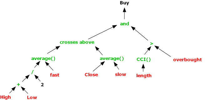
Genetic programming is an evolutionary-based algorithmic methodology which can be used in a very general way to identify patterns or rules within data structures. The GP system is given a set of instructions (typically simple operators like addition and subtraction), some data observations and a fitness function to assess how well the system is able to combine the functions and data to achieve a specified goal.

In the trading strategy context the data observations might include not only price data, but also price volatility, moving averages and a variety of other technical indicators. The fitness function could be something as simple as net profit, but might represent alternative measures of profitability or risk, with factors such as PL per trade, win rate, or maximum drawdown. In order to reduce the danger of over-fitting, it is customary to limit the types of functions that the system can use to simple operators (+,-,/,*), exponents, and trig functions. The length of the program might also be constrained in terms of the maximum permitted lines of code.

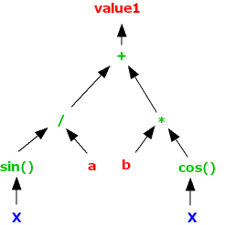
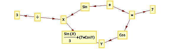
We can represent what is going on using a tree graph:

In this example the GP system is combining several simple operators with the Sin and Cos trig functions to create a signal comprising an expression in two variables, X and Y, which may be, for example, stock prices, moving averages, or technical indicators of momentum or mean reversion.
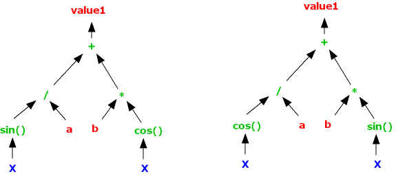
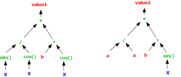
The “evolutionary” aspect of the GP process derives from the idea that an existing signal or model can be mutated by replacing nodes in a branch of a tree, or even an entire branch by another. System performance is re-evaluated using the fitness function and the most profitable mutations are retained for further generation.
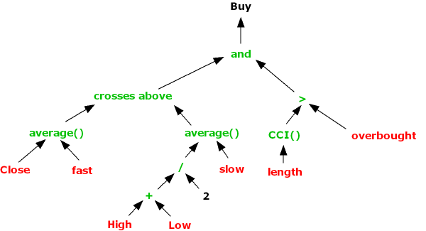
The resulting models are often highly non-linear and can be very general in form.

A GP Daytrading Strategy
The last fifteen years has seen tremendous advances in the field of genetic programming, in terms of the theory as well as practice. Using a single hyper-threaded CPU, it is now possible for a GP system to generate signals at a far faster rate than was possible on Proteom’s cluster of 50 networked CPUs. A researcher can develop and evaluate tens of millions of possible trading algorithms with the space of a few hours. Implementing a thoroughly researched and tested strategy is now feasible in a matter of weeks. There can be no doubt of GP’s potential to produce dramatic reductions in R&D lead times and costs. But does it work?

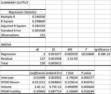
To address that question I have summarized below the performance results from a GP-developed daytrading system that trades nine different futures markets: Crude Oil (CL), Euro (EC), E-Mini (ES), Gold (GC), Heating Oil (HO), Coffee (KC), Natural gas (NG), Ten Year Notes (TY) and Bonds (US). The system trades a single contract in each market individually, going long and short several times a day. Only the most liquid period in each market is traded, which typically coincides with the open-outcry session, with any open positions being exited at the end of the session using market orders. With the exception of the NG and HO markets, which are entered using stop orders, all of the markets are entered and exited using standard limit orders, at prices determined by the system

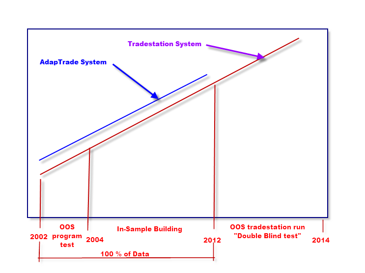
The system was constructed using 15-minute bar data from Jan 2006 to Dec 2011 and tested out-of-sample of data from Jan 2012 to May 2014. The in-sample span of data was chosen to cover periods of extreme market stress, as well as less volatile market conditions. A lengthy out-of-sample period, almost half the span of the in-sample period, was chosen in order to evaluate the robustness of the system.
Out-of-sample testing was “double-blind”, meaning that the data was not used in the construction of the models, nor was out-of-sample performance evaluated by the system before any model was selected.

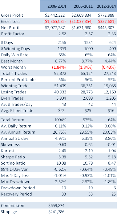
Performance results are net of trading commissions of $6 per round turn and, in the case of HO and NG, additional slippage of 2 ticks per round turn.

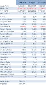
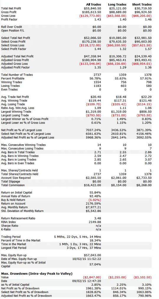
(click on the table for a higher definition view)

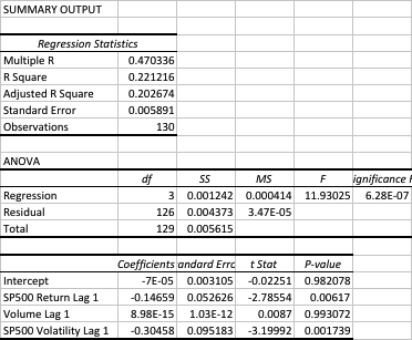
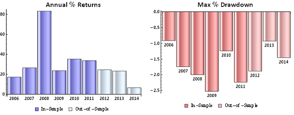
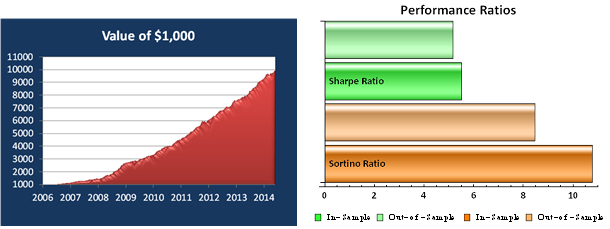
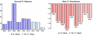
The most striking feature of the strategy is the high rate of risk-adjusted returns, as measured by the Sharpe ratio, which exceeds 5 in both in-sample and out-of-sample periods. This consistency is a reflection of the fact that, while net returns fall from an annual average of over 29% in sample to around 20% in the period from 2012, so, too, does the strategy volatility decline from 5.35% to 3.86% in the respective periods. The reduction in risk in the out-of-sample period is also reflected in lower Value-at-Risk and Drawdown levels.

A decline in the average PL per trade from $25 to $16 in offset to some degree by a slight increase in the rate of trading, from 42 to 44 trades per day, on average, while daily win rate and percentage profitable trades remain consistent at around 65% and 56%, respectively.

Overall, the system appears to be not only highly profitable, but also extremely robust. This is impressive, given that the models were not updated with data after 2011, remaining static over a period almost half as long as the span of data used in their construction. It is reasonable to expect that out-of-sample performance might be improved by allowing the models to be updated with more recent data.

Benefits and Risks of the GP Approach to Trading System Development
The potential benefits of the GP approach to trading system development include speed of development, flexibility of design, generality of application across markets and rapid testing and deployment.

What about the downside? The most obvious concern is the risk of over-fitting. By allowing the system to develop and test millions of models, there is a distinct risk that the resulting systems may be too closely conditioned on the in-sample data, and will fail to maintain performance when faced with new market conditions. That is why, of course, we retain a substantial span of out-of-sample data, in order to evaluate the robustness of the trading system. Even so, given the enormous number of models evaluated, there remains a significant risk of over-fitting.

Another drawback is that, due to the nature of the modelling process, it can be very difficult to understand, or explain to potential investors, the “market hypothesis” underpinning any specific model. “We tested it and it works” is not a particularly enlightening explanation for investors, who are accustomed to being presented with a more articulate theoretical framework, or investment thesis. Not being able to explain precisely how a system makes money is troubling enough in good times; but in bad times, during an extended drawdown, investors are likely to become agitated very quickly indeed if no explanation is forthcoming. Unfortunately, evaluating the question of whether a period of poor performance is temporary, or the result of a breakdown in the model, can be a complicated process.

Finally, in comparison with other modeling techniques, GP models suffer from an inability to easily update the model parameters based on new data as it become available. Typically, as GP model will be to rebuilt from scratch, often producing very different results each time.

Conclusion
Despite the many limitations of the GP approach, the advantages in terms of the speed and cost of researching and developing original trading signals and strategies have become increasingly compelling.

Given the several well-documented successes of the GP approach in fields as diverse as genetics and physics, I think an appropriate position to take with respect to applications within financial market research would be one of cautious optimism.
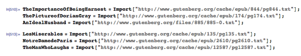
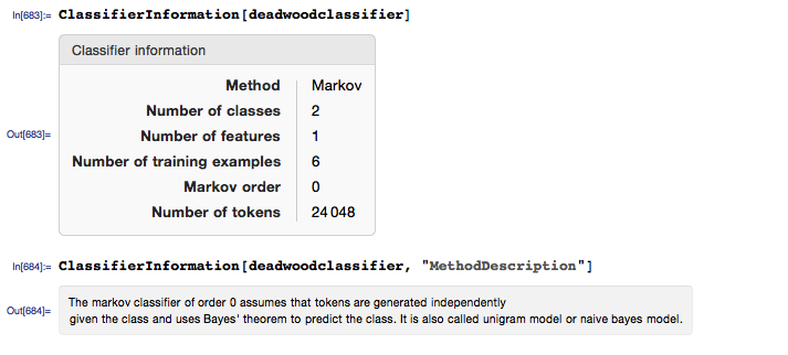
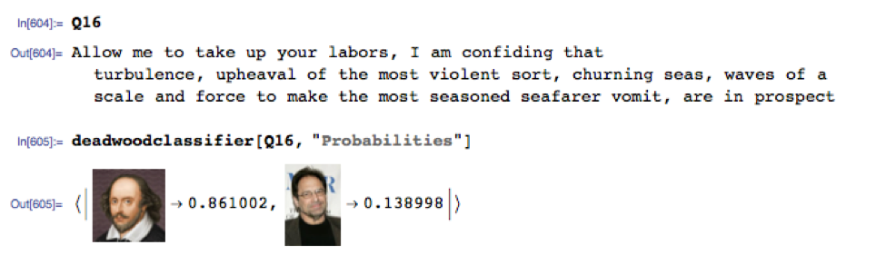
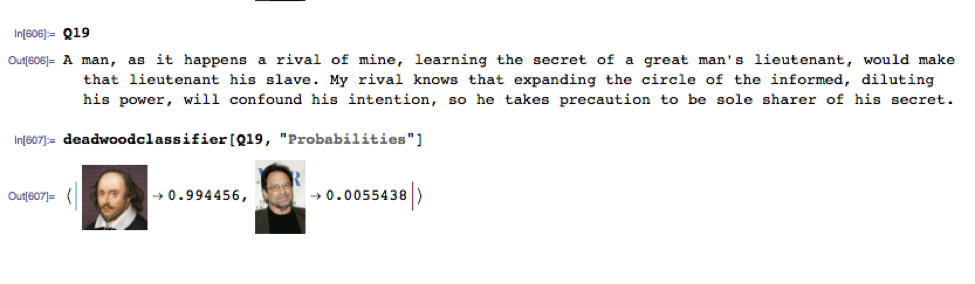
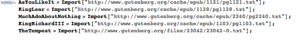