
The Story of a HFT Strategy


QUANTITATIVE RESEARCH AND TRADING
The latest theories, models and investment strategies in quantitative research and trading

Continuing a previous post, in which we modeled the relationship in the levels of the VIX Index and the Year 1 and Year 2 CBOE Correlation Indices, we next turn our attention to modeling changes in the VIX index.
In case you missed it, the post can be found here:
http://jonathankinlay.com/2017/08/correlation-cointegration/
We saw previously that the levels of the three indices are all highly correlated, and we were able to successfully account for approximately half the variation in the VIX index using either linear regression models or non-linear machine-learning models that incorporated the two correlation indices. It turns out that the log-returns processes are also highly correlated:

We can create a simple linear regression model that relates log-returns in the VIX index to contemporaneous log-returns in the two correlation indices, as follows. The derived model accounts for just under 40% of the variation in VIX index returns, with each correlation index contributing approximately one half of the total VIX return.

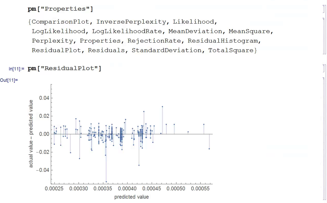
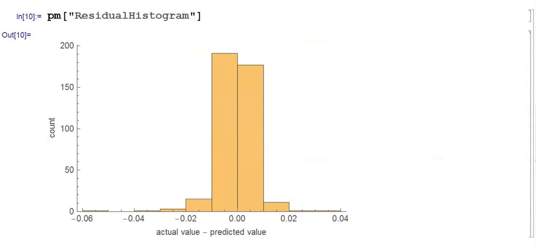
Although the linear model is highly statistically significant, we see clear evidence of lack of fit in the model residuals, which indicates non-linearities present in the relationship. So, ext we use a nearest-neighbor algorithm, a machine learning technique that allows us to model non-linear components of the relationship. The residual plot from the nearest neighbor model clearly shows that it does a better job of capturing these nonlinearities, with lower standard in the model residuals, compared to the linear regression model:

Another approach entails the use of copulas to model the inter-dependency between the volatility and correlation indices. For a fairly detailed exposition on copulas, see the following blog posts:
http://jonathankinlay.com/2017/01/copulas-risk-management/
http://jonathankinlay.com/2017/03/pairs-trading-copulas/
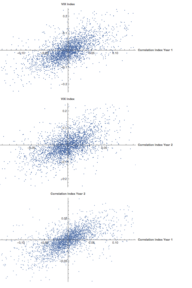
We begin by taking a smaller sample comprising around three years of daily returns in the indices. This minimizes the impact of any long-term nonstationarity in the processes and enables us to fit marginal distributions relatively easily. First, let’s look at the correlations in our sample data:

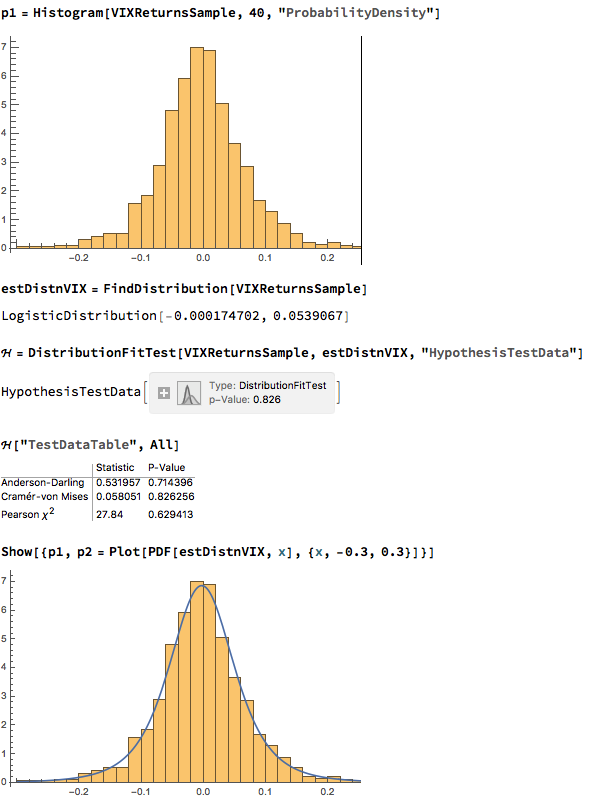
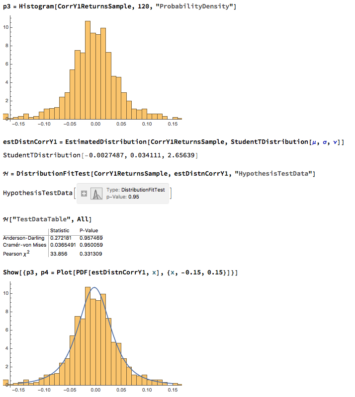
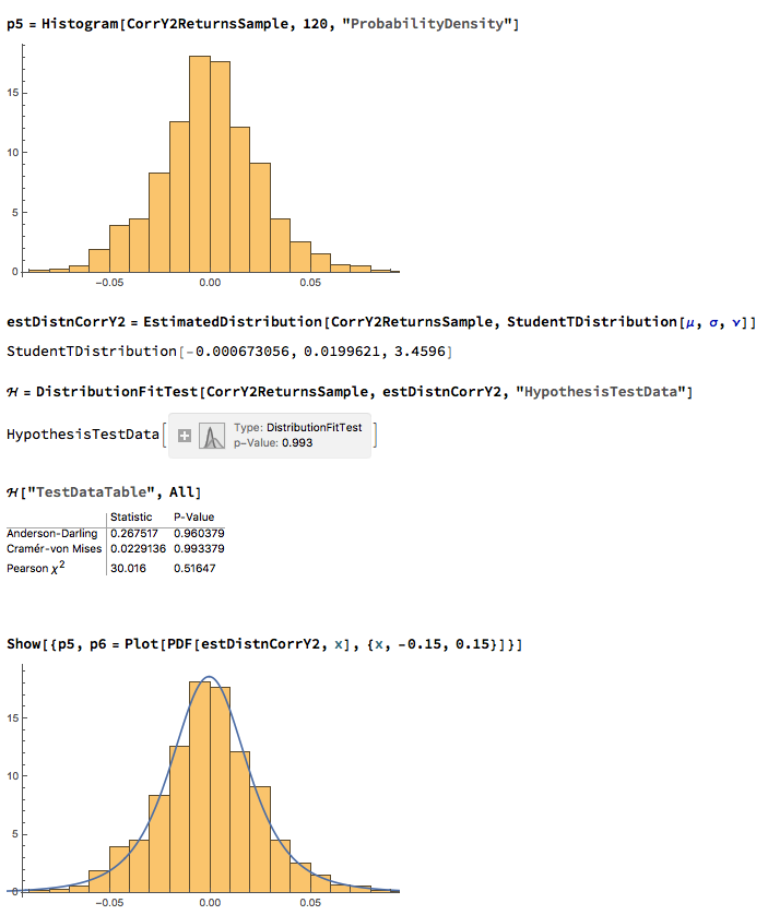
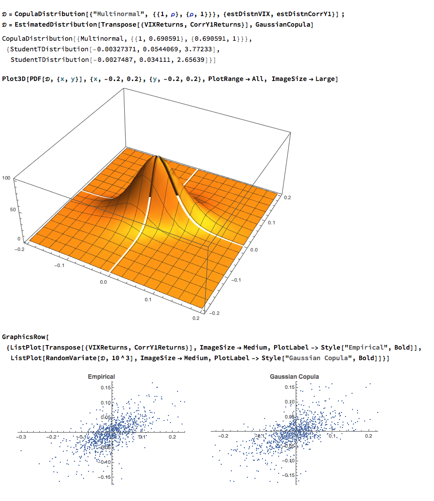
We next proceed to fit margin distributions to the VIX and Correlation Index processes. It turns out that the VIX process is well represented by a Logistic distribution, while the two Correlation Index returns processes are better represented by a Student-T density. In all three cases there is little evidence of lack of fit, wither in the body or tails of the estimated probability density functions:
The final step is to fit a copula to model the joint density between the indices. To keep it simple I have chosen to carry out the analysis for the combination of the VIX index with only the first of the correlation indices, although in principle there no reason why a copula could not be estimated for all three indices. The fitted model is a multinormal Gaussian copula with correlation coefficient of 0.69. of course, other copulas are feasible (Clayton, Gumbel, etc), but Gaussian model appears to provide an adequate fit to the empirical copula, with approximate symmetry in the left and right tails.

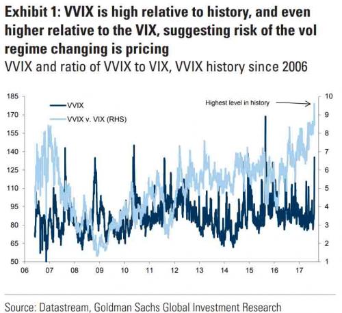
In a previous blog post I mentioned the VVIX/VIX Ratio, which is measured as the ratio of the CBOE VVIX Index to the VIX Index. The former measures the volatility of the VIX, or the volatility of volatility.
http://jonathankinlay.com/2017/07/market-stress-test-signals-danger-ahead/
A follow-up article in ZeroHedge shortly afterwards pointed out that the VVIX/VIX ratio had reached record highs, prompting Goldman Sachs analyst Ian Wright to comment that this could signal the ending of the current low-volatility regime:
A linkedIn reader pointed out that individual stock volatility was currently quite high and when selling index volatility one is effectively selling stock correlations, which had now reached historically low levels. I concurred:
What’s driving the low vol regime is the exceptionally low level of cross-sectional correlations. And, as correlations tighten, index vol will rise. Worse, we are likely to see a feedback loop – higher vol leading to higher correlations, further accelerating the rise in index vol. So there is a second order, Gamma effect going on. We see that is the very high levels of the VVIX index, which shot up to 130 last week. The all-time high in the VVIX prior to Aug 2015 was around 120. The intra-day high in Aug 2015 reached 225. I’m guessing it will get back up there at some point, possibly this year.
As there appears to be some interest in the subject I decided to add a further blog post looking a little further into the relationship between volatility and correlation. To gain some additional insight we are going to make use of the CBOE implied correlation indices. The CBOE web site explains:
Using SPX options prices, together with the prices of options on the 50 largest stocks in the S&P 500 Index, the CBOE S&P 500 Implied Correlation Indexes offers insight into the relative cost of SPX options compared to the price of options on individual stocks that comprise the S&P 500.
- CBOE calculates and disseminates two indexes tied to two different maturities, usually one year and two years out. The index values are published every 15 seconds throughout the trading day.
- Both are measures of the expected average correlation of price returns of S&P 500 Index components, implied through SPX option prices and prices of single-stock options on the 50 largest components of the SPX.
One application is dispersion trading, which the CBOE site does a good job of summarizing:
The CBOE S&P 500 Implied Correlation Indexes may be used to provide trading signals for a strategy known as volatility dispersion (or correlation) trading. For example, a long volatility dispersion trade is characterized by selling at-the-money index option straddles and purchasing at-the-money straddles in options on index components. One interpretation of this strategy is that when implied correlation is high, index option premiums are rich relative to single-stock options. Therefore, it may be profitable to sell the rich index options and buy the relatively inexpensive equity options.
Again, the CBOE web site is worth quoting:
The CBOE S&P 500 Implied Correlation Indexes measure changes in the relative premium between index options and single-stock options. A single stock’s volatility level is driven by factors that are different from what drives the volatility of an Index (which is a basket of stocks). The implied volatility of a single-stock option simply reflects the market’s expectation of the future volatility of that stock’s price returns. Similarly, the implied volatility of an index option reflects the market’s expectation of the future volatility of that index’s price returns. However, index volatility is driven by a combination of two factors: the individual volatilities of index components and the correlation of index component price returns.
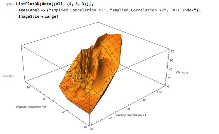
Let’s dig into this analytically. We first download and plot the daily for the VIX and Correlation Indices from the CBOE web site, from which it is evident that all three series are highly correlated:
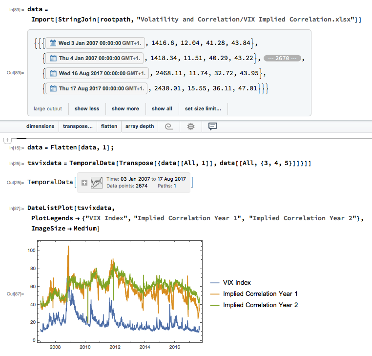
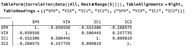
An inspection reveals significant correlations between the VIX index and the two implied correlation indices, which are themselves highly correlated. The S&P 500 Index is, of course, negatively correlated with all three indices:
The response surface that describes the relationship between the VIX index and the two implied correlation indices is locally very irregular, but the slope of the surface is generally positive, as we would expect, since the level of VIX correlates positively with that of the two correlation indices.
The most straightforward approach is to use a simple linear regression specification to model the VIX level as a function of the two correlation indices. We create a VIX Model Surface object using this specification with the Mathematica Predict function: The linear model does quite a good job of capturing the positive gradient of the response surface, and in fact has a considerable amount of explanatory power, accounting for a little under half the variance in the level of the VIX index:
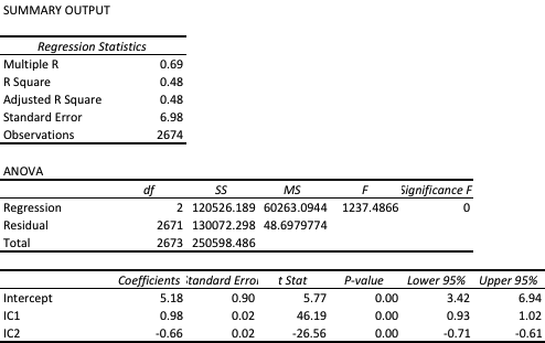
However, there are limitations. To begin with, the assumption of independence between the explanatory variables, the correlation indices, clearly does not hold. In cases such as this, where explanatory variables are multicolinear, we are unable to draw inferences about the explanatory power of individual regressors, even though the model as a whole may be highly statistically significant, as here.
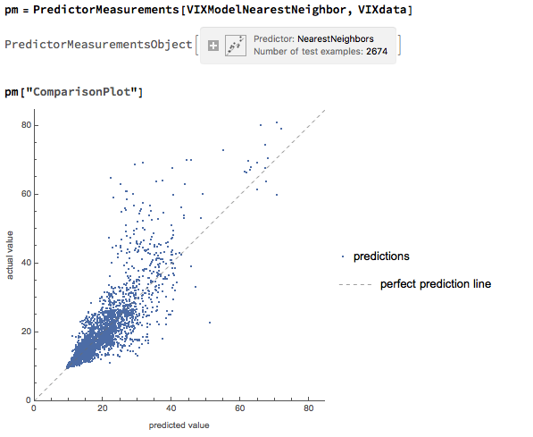
Secondly, a linear regression model is not going to capture non-linearities in the volatility-correlation relationship that are evident in the surface plot. This is confirmed by a comparison plot, which shows that the regression model underestimates the VIX level for both low and high values of the index:

We can achieve a better outcome using a machine learning algorithm such as nearest neighbor, which is able to account for non-linearities in the response surface:

The comparison plot shows a much closer correspondence between actual and predicted values of the VIX index, even though there is evidence of some remaining heteroscedasticity in the model residuals:
A useful way to think about index volatility is as a two dimensional process, with time-series volatility measured on one dimension and dispersion (cross-sectional volatility, the inverse of correlation) measured on the second. The two factors are correlated and, as we have shown here, interact in a complicated, non-linear way.
The low levels of index volatility we have seen in recent months result, not from low levels of volatility in component stocks, but in the historically low levels of correlation (high levels of dispersion) in the underlying stock returns processes. As correlations begin to revert to historical averages, the impact will be felt in an upsurge in index volatility, compounded by the non-linear interaction between the two factors.

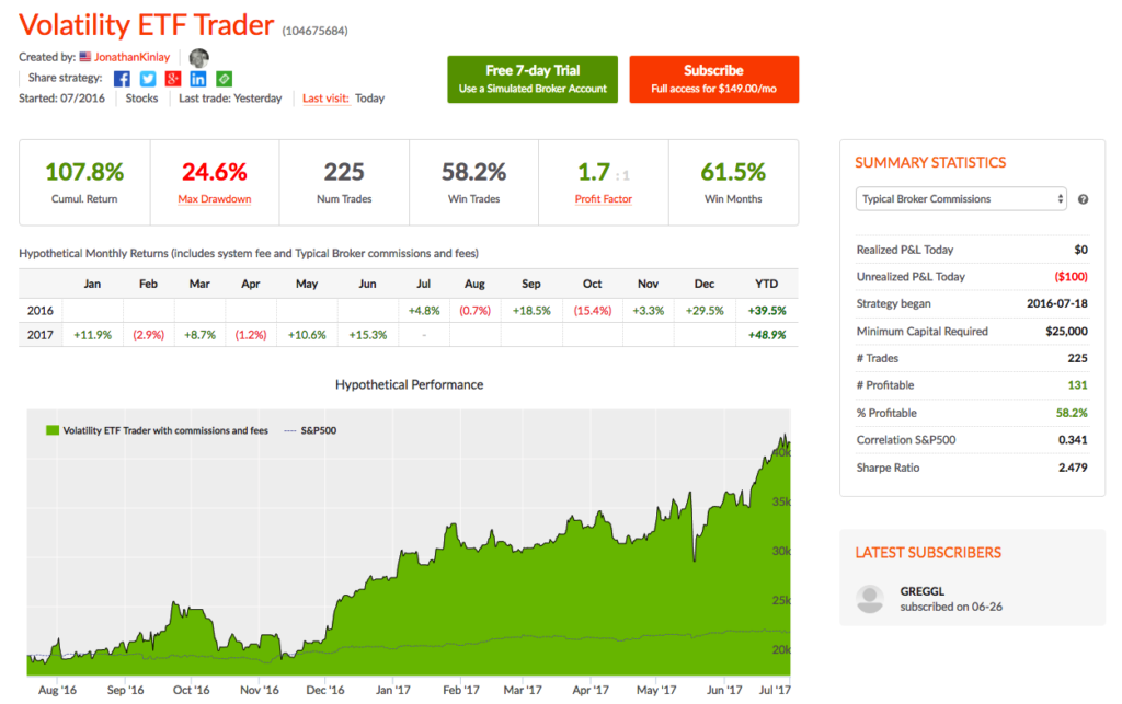
The Volatility ETF Trader product is an algorithmic strategy that trades several VIX ETFs using statistical and machine learning algorithms.
We offer a version of the strategy on the Collective 2 site (see here for details) that the user can subscribe to for a very modest fee of only $149 per month.
The risk-adjusted performance of the Collective 2 version of the strategy is unlikely to prove as good as the product we offer in our Systematic Strategies Fund, which trades a much wider range of algorithmic strategies. There are other important differences too: the Fund’s Systematic Volatility Strategy makes no use of leverage and only trades intra-day, exiting all positions by market close. So it has a more conservative risk profile, suitable for longer term investment.
The Volatility ETF Trader on Collective 2, on the other hand, is a highly leveraged, tactical strategy that trades positions overnight and holds them for periods of several days . As a consequence, the Collective 2 strategy is far more risky and is likely to experience significant drawdowns. Those caveats aside, the strategy returns have been outstanding: +48.9% for 2017 YTD and a total of +107.8% from inception in July 2016.
You can find full details of the strategy, including a listing of all of the trades, on the Collective 2 site.
Subscribers can sign up for a free, seven day trial and thereafter they can choose to trade the strategy automatically in their own brokerage account.

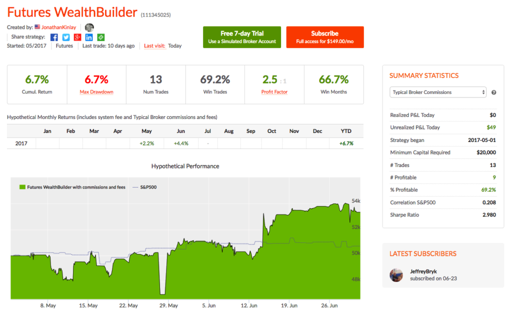
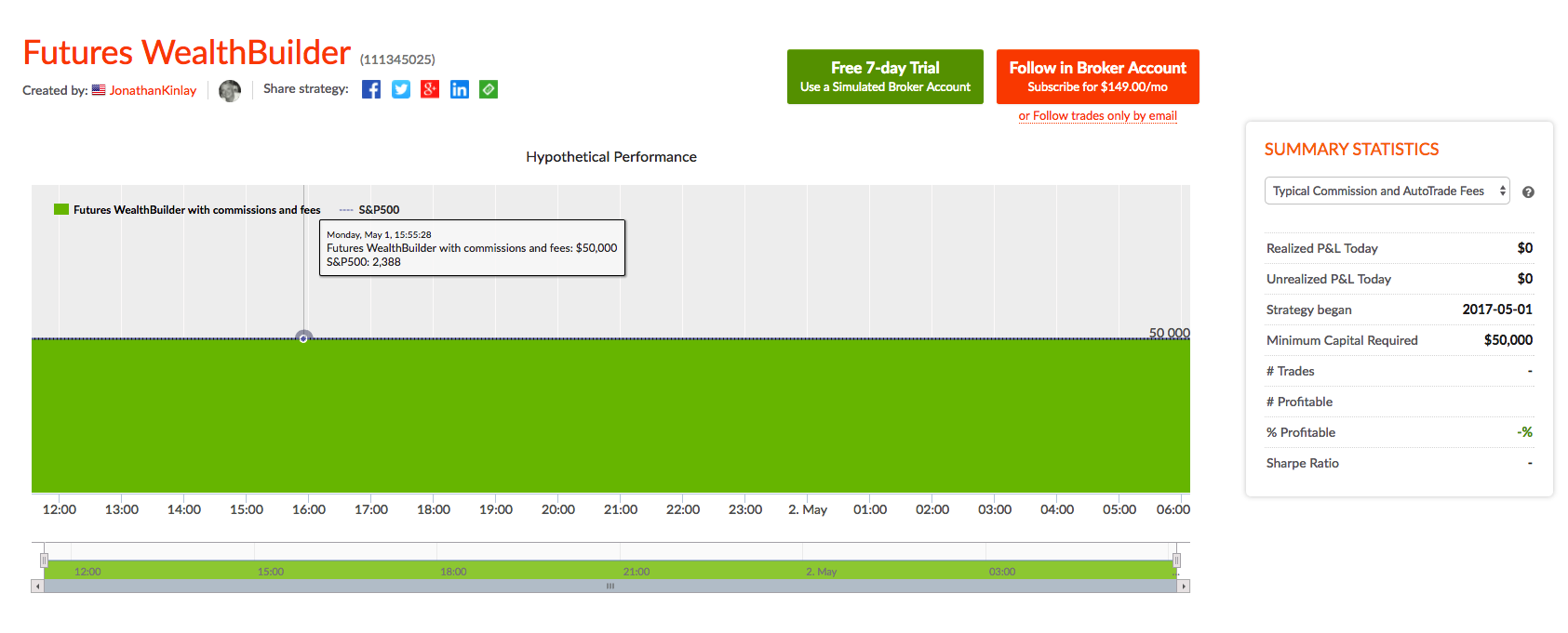
The Futures WealthBuilder product is an algorithmic CTA strategy that trades several highly liquid futures contracts using machine learning algorithms. More details about the strategy are given in this blog post.
We offer a version of the strategy on the Collective 2 site (see here for details) that the user can subscribe to for a very modest fee of only $149 per month. The Collective 2 version of the strategy is unlikely to perform as well as the product we offer in our Systematic Strategies Fund, which trades a much wider range of futures products. But the strategy is off to an excellent start, making +4.4% in June and is now up 6.7% since inception in May. In June the strategy made profitable trades in US Bonds, Euro F/X and VIX futures, and the last seven trades in a row have been winners.
You can find full details of the strategy, including a listing of all of the trades, on the Collective 2 site.
Subscribers can sign up for a free, seven day trial and thereafter they can choose to trade the strategy automatically in their own brokerage account, using the Collective 2 api.

We are launching a new product, the Futures WealthBuilder, a CTA system that trades futures contracts in several highly liquid financial and commodity markets, including SP500 EMinis, Euros, VIX, Gold, US Bonds, 10-year and five-year notes, Corn, Natural Gas and Crude Oil. Each component strategy uses a variety of machine learning algorithms to detect trends, seasonal effects and mean-reversion. We develop several different types of model for each market, and deploy them according to their suitability for current market conditions.
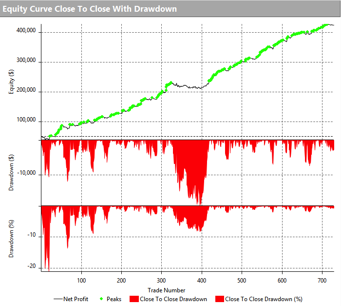
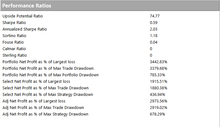
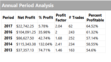
Performance of the strategy (net of fees) since 2013 is detailed in the charts and tables below. Notable features include a Sharpe Ratio of just over 2, an annual rate of return of 190% on an account size of $50,000, and a maximum drawdown of around 8% over the last three years. It is worth mentioning, too, that the strategy produces approximately equal rates of return on both long and short trades, with an overall profit factor above 2.


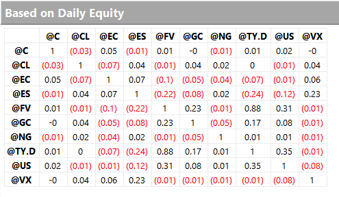
Despite a high level of correlation between several of the underlying markets, the correlation between the component strategies of Futures WealthBuilder are, in the majority of cases, negligibly small (with a few exceptions, such as the high correlation between the 10-year and 5-year note strategies). This accounts for the relative high level of return in relation to portfolio risk, as measured by the Sharpe Ratio. We offer strategies in both products chiefly as a mean of providing additional liquidity, rather than for their diversification benefit.
Strategy robustness is a key consideration in the design stage. We use Monte Carlo simulation to evaluate scenarios not seen in historical price data in order to ensure consistent performance across the widest possible range of market conditions. Our methodology introduces random fluctuations to historical prices, increasing or decreasing them by as much as 30%. We allow similar random fluctuations in that value strategy parameters, to ensure that our models perform consistently without being overly-sensitive to the specific parameter values we have specified. Finally, we allow the start date of each sub-system to vary randomly by up to a year.
The effect of these variations is to produce a wide range of outcomes in terms of strategy performance. We focus on the 5% worst outcomes, ranked by profitability, and select only those strategies whose performance is acceptable under these adverse scenarios. In this way we reduce the risk of overfitting the models while providing more realistic expectations of model performance going forward. This procedure also has the effect of reducing portfolio tail risk, and the maximum peak-to-valley drawdown likely to be produced by the strategy in future.

We will be running a variant of the Futures WealthBuilder strategy on the Collective 2 site, using a subset of the strategy models in several futures markets(see this page for details). Subscribers will be able to link and auto-trade the strategy in their own account, assuming they make use of one of the approved brokerages which include Interactive Brokers, MB Trading and several others.
Obviously the performance is unlikely to be as good as the complete strategy, since several component sub-strategies will not be traded on Collective 2. However, this does give the subscriber the option to trial the strategy in simulation before plunging in with real money.


Text and sentiment analysis has become a very popular topic in quantitative research over the last decade, with applications ranging from market research and political science, to e-commerce. In this post I am going to outline an approach to the subject, together with some core techniques, that have applications in investment strategy.
In the early days of the developing field of market sentiment analysis, the supply of machine readable content was limited to mainstream providers of financial news such as Reuters or Bloomberg. Over time this has changed with the entry of new competitors in the provision of machine readable news, including, for example, Ravenpack or more recent arrivals like Accern. Providers often seek to sell not only the raw news feed service, but also their own proprietary sentiment indicators that are claimed to provide additional insight into how individual stocks, market sectors, or the overall market are likely to react to news. There is now what appears to be a cottage industry producing white papers seeking to demonstrate the value of these services, often accompanied by some impressive pro-forma performance statistics for the accompanying strategies, which include long-only, long/short, market neutral and statistical arbitrage.
For the purpose of demonstration I intend to forego the blandishments of these services, although many are no doubt are excellent, since the reader is perhaps unlikely to have access to them. Instead, in what follows I will focus on a single news source, albeit a highly regarded one: the Wall Street Journal. This is, of course, a simplification intended for illustrative purposes only – in practice one would need to use a wide variety of news sources and perhaps subscribe to a machine readable news feed service. But similar principles and techniques can be applied to any number of news feeds or online sites.
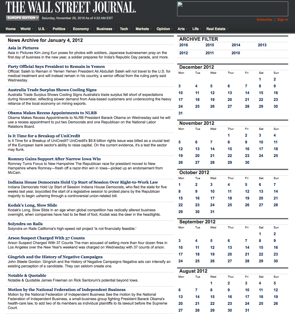
We are going to access the Journal’s online archive, which presents daily news items in a convenient summary format, an example of which is shown below. The archive runs from the beginning of 2012 through to the current day, providing ample data for analysis. In what follows, I am going to make two important assumptions, neither of which is likely to be 100% accurate – but which will not detract too much from the validity of the research, I hope. The first assumption is that the news items shown in each daily archive were reported prior to the market open at 9:30 AM. This is likely to be true for the great majority of the stories, but there are no doubt important exceptions. Since we intend to treat the news content of each archive as antecedent to the market action during the corresponding trading session, exceptions are likely to introduce an element of look-ahead bias. The second assumption is that the archive for each day is shown in the form in which it would have appeared on the day in question. In reality, there are likely to have been revisions to some of the stories made subsequent to their initial publication. So, here too, we must allow for the possibility of look-ahead bias in the ensuing analysis.
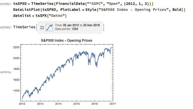
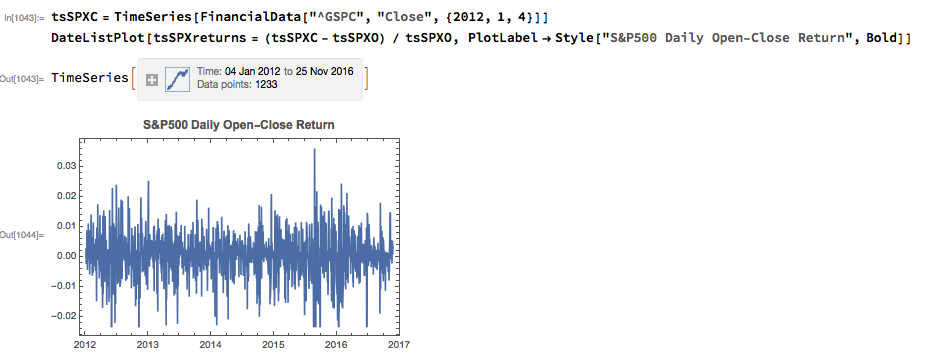
With those caveats out of the way, let’s proceed. We are going to be using broad market data for the S&P 500 index in the analysis to follow, so the first step is to download daily price series for the index. Note that we begin with daily opening prices, since we intend to illustrate the application of news sentiment analysis with a theoretical day-trading strategy that takes positions at the start of each trading session, exiting at market close.
From there we calculate the intraday return in the index, from market open to close, as follows:
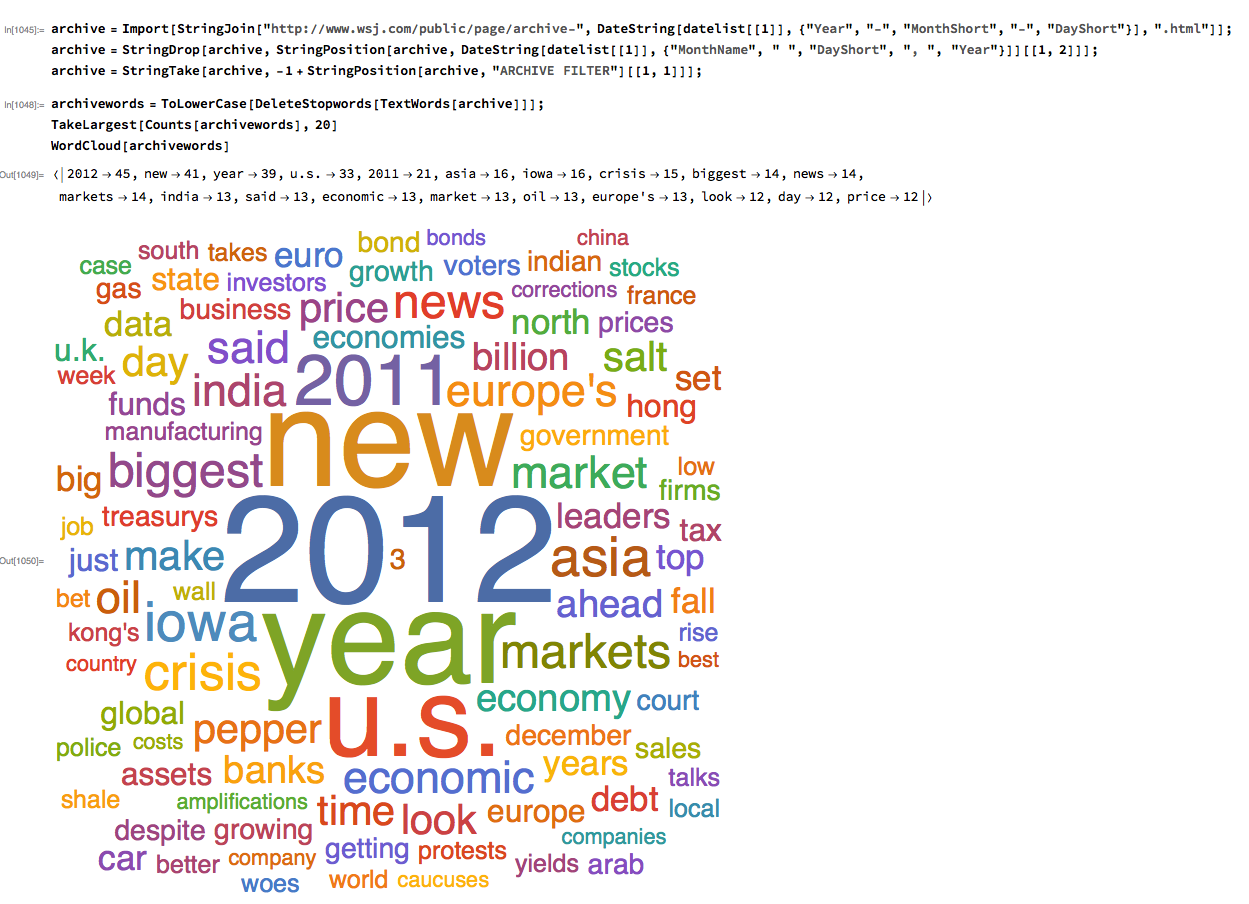
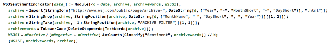
Next we turn to the task of reading the news archive and categorizing its content. Mathematica makes the importation of html pages very straightforward, and we can easily crop the raw text string to exclude page headers and footers. The approach I am going to take is to derive a sentiment indicator based on an analysis of the sentiment of each word in the daily archive. Before we can do that we must first convert the text into individuals words, stripping out standard stop-words such as “the” and “in” and converting all the text to lower case. Naturally one can take this pre-processing a great deal further, by identifying and separating out proper nouns, for example. Once the text processing stage is complete we can quickly summarize the content, for example by looking at the most common words, or by representing the entire archive in the form of a word cloud. Given that we are using the archive for the first business day of 2012, it is perhaps unsurprising that we find that “2012”, “new” and “year” feature so prominently!
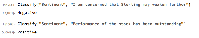
The subject of sentiment analysis is a complex one and I only touch on it here. For those interested in the subject I can recommend The Text Mining Handbook, by Feldman and Sanger, which is a standard work on the topic. Here I am going to employ a machine learning classifier provided with Mathematica 11. It is not terribly sophisticated (or, at least, has not been developed with financial applications especially in mind), but will serve for the purposes of this article. For those unfamiliar with the functionality, the operation of the sentiment classification algorithm is straightforward enough. For instance:
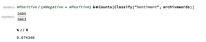
We apply the algorithm to classify each word in the daily news archive and arrive at a sentiment indicator based on the proportion of words that are classified as “positive”. The sentiment reading for the archive for Jan-3, 2012, for example, turns out to be 67.4%:
We can automate the process of classifying the entire WSJ archive with just a few lines of code, producing a time series for the daily sentiment indicator, which has an average daily value of 68.5% – the WSJ crowd tends to be bullish, clearly! Note how the 60-day moving average of the indicator rises steadily over the period from 2012 through Q1 2015, then abruptly reverses direction, declining steadily thereafter – even somewhat precipitously towards the end of 2016.

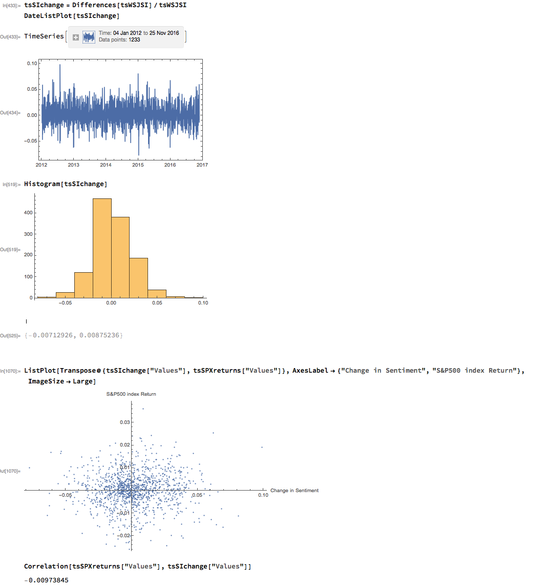
As with most data series in investment research, we are less interested in the level of a variable, such as a stock price, than we are in the changes in level. So the next step is to calculate the daily percentage change in the sentiment indicator and examine the correlation with the corresponding intraday return in the S&P 500 Index. At first glance our sentiment indicator appears to have very little predictive power – the correlation between indicator changes and market returns is negligibly small overall – but we shall later see that this is not the last word.
Thus far the results appear discouraging; but as is often the case with this type of analysis we need to look more closely at the conditional distribution of returns. Specifically, we will examine the conditional distribution of S&P 500 Index returns when changes in the sentiment index are in the upper and lower quantiles of the distribution. This will enable us to isolate the impact of changes in market sentiment at times when the swings in sentiment are strongest. In the analysis below, we begin by examining the upper and lower third of the distribution of changes in sentiment:
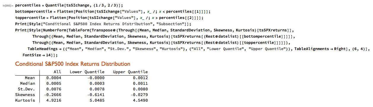
The analysis makes clear that the distribution of S&P 500 Index returns is very different on days when the change in market sentiment is large and positive vs. large and negative. The difference is not just limited to the first moment of the conditional distribution, where the difference in the mean return is large and statistically significant, but also in the third moment. The much larger, negative skewness means that there is a greater likelihood of a large decline in the market on days in which there is a sizable drop in market sentiment, than on days in which sentiment significantly improves. In other words, the influence of market sentiment changes is manifest chiefly through the mean and skewness of the conditional distributions of market returns.
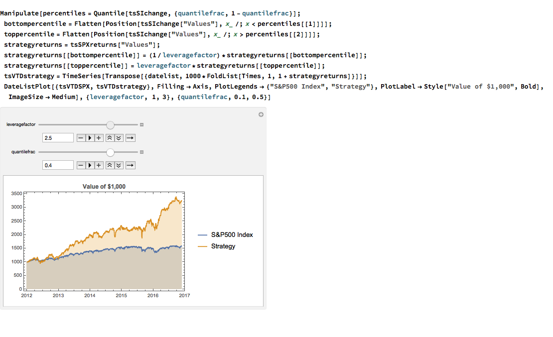
We can capitalize on these effects using a simple trading strategy in which we increase the capital allocated to a long-SPX position on days when market sentiment improves, while reducing exposure on days when market sentiment falls. We increase the allocation by a factor – designated the leverage factor – on days when the change in the sentiment indicator is in the upper 1/3 of the distribution, while reducing the allocation by 1/leveragefactor on days when the change in the sentiment indicator falls in lower 1/3 of the distribution. The allocation on other days is 100%. The analysis runs as follows:

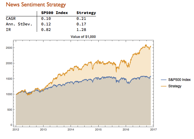
It turns out that, using a leverage factor of 2.0, we can increase the CAGR from 10% to 21% over the period from 2012-2016 using the conditional distribution approach. This performance enhancement comes at a cost, since the annual volatility of the news sentiment strategy is 17% compared to only 12% for the long-only strategy. However, the overall net result is positive, since the risk-adjusted rate of return increases from 0.82 to 1.28.
We can explore the robustness of the result, comparing different quantile selections and leverage factors using Mathematica’s interactive Manipulate function:
We have seen that a simple market sentiment indicator can be created quite easily from publicly available news archives, using a standard machine learning sentiment classification algorithm. A market sentiment algorithm constructed using methods as straightforward as this appears to provide the capability to differentiate the conditional distribution of market returns on days when changes in market sentiment are significantly positive or negative. The differences in the higher moments of the conditional distribution appears to be as significant as the differences in the mean. In principle, we can use the insight provided by the sentiment indicator to enhance a long-only day-trading strategy, increasing leverage and allocation on days when changes to market sentiment are positive and reducing them on days when sentiment declines. The performance enhancements resulting from this approach appear to be significant.
Several caveats apply. The S&P 500 index is not tradable, of course, and it is not uncommon to find trading strategies that produce interesting theoretical results. In practice one would be obliged to implement the strategy using a tradable market proxy, such as a broad market ETF or futures contract. The strategy described here, which enters and exits positions daily, would incur substantial trading costs, that would be further exacerbated by the use of leverage.
Of course there are many other uses one can make of news data, in particular with firm-specific news and sentiment analytics, that fall outside the scope of this article. Hopefully, however, the methodology described here will provide a sign-post towards further, more practically useful research.


The SPDR S&P 500 ETF (SPY) is one of the widely traded ETF products on the market, with around $200Bn in assets and average turnover of just under 200M shares daily. So the likelihood of being able to develop a money-making trading system using publicly available information might appear to be slim-to-none. So, to give ourselves a fighting chance, we will focus on an attempt to predict the overnight movement in SPY, using data from the prior day’s session.
In addition to the open/high/low and close prices of the preceding day session, we have selected a number of other plausible variables to build out the feature vector we are going to use in our machine learning model:
We will attempt to build a model that forecasts the overnight return in the ETF, i.e. [O(t+1)-C(t)] / C(t)
In this exercise we use daily data from the beginning of the SPY series up until the end of 2014 to build the model, which we will then test on out-of-sample data running from Jan 2015-Aug 2016. In a high frequency context a considerable amount of time would be spent evaluating, cleaning and normalizing the data. Here we face far fewer problems of that kind. Typically one would standardized the input data to equalize the influence of variables that may be measured on scales of very different orders of magnitude. But in this example all of the input variables, with the exception of volume, are measured on the same scale and so standardization is arguably unnecessary.
First, the in-sample data is loaded and used to create a training set of rules that map the feature vector to the variable of interest, the overnight return:
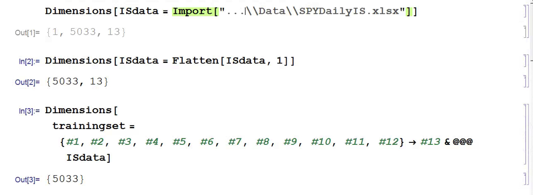
In Mathematica 10 Wolfram introduced a suite of machine learning algorithms that include regression, nearest neighbor, neural networks and random forests, together with functionality to evaluate and select the best performing machine learning technique. These facilities make it very straightfoward to create a classifier or prediction model using machine learning algorithms, such as this handwriting recognition example:

We create a predictive model on the SPY trainingset, allowing Mathematica to pick the best machine learning algorithm:

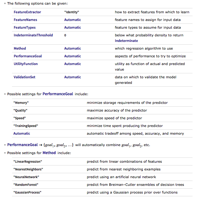
There are a number of options for the Predict function that can be used to control the feature selection, algorithm type, performance type and goal, rather than simply accepting the defaults, as we have done here:
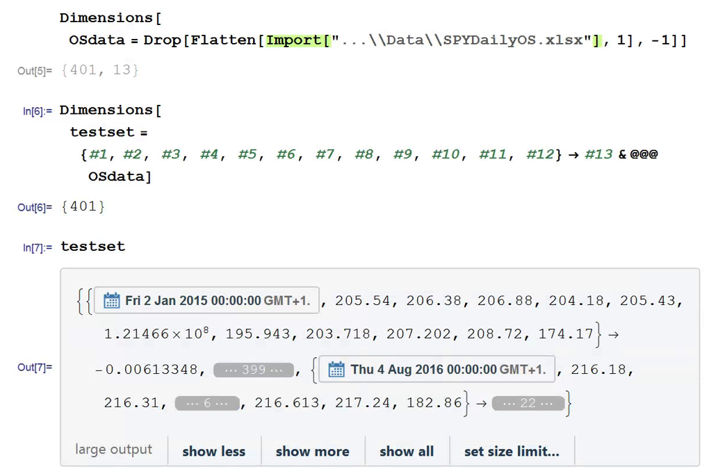
Having built our machine learning model, we load the out-of-sample data from Jan 2015 to Aug 2016, and create a test set:
We next create a PredictionMeasurement object, using the Nearest Neighbor model , that can be used for further analysis:
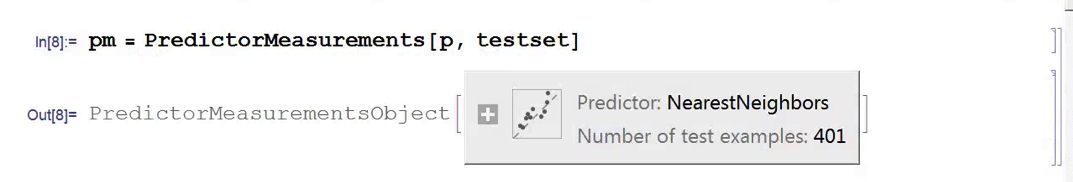
There isn’t much dispersion in the model forecasts, which all have positive value. A common technique in such cases is to subtract the mean from each of the forecasts (and we may also standardize them by dividing by the standard deviation).
The scatterplot of actual vs. forecast overnight returns in SPY now looks like this:

There’s still an obvious lack of dispersion in the forecast values, compared to the actual overnight returns, which we could rectify by standardization. In any event, there appears to be a small, nonlinear relationship between forecast and actual values, which holds out some hope that the model may yet prove useful.
There are various methods of deploying a forecasting model in the context of creating a trading system. The simplest route, which we will take here, is to apply a threshold gate and convert the filtered forecasts directly into a trading signal. But other approaches are possible, for example:
In this example we will create a trading model by applying a simple filter to the forecasts, picking out only those values that exceed a specified threshold. This is a standard trick used to isolate the signal in the model from the background noise. We will accept only the positive signals that exceed the threshold level, creating a long-only trading system. i.e. we ignore forecasts that fall below the threshold level. We buy SPY at the close when the forecast exceeds the threshold and exit any long position at the next day’s open. This strategy produces the following pro-forma results:
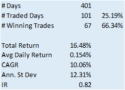

The system has some quite attractive features, including a win rate of over 66% and a CAGR of over 10% for the out-of-sample period.
Obviously, this is a very basic illustration: we would want to factor in trading commissions, and the slippage incurred entering and exiting positions in the post- and pre-market periods, which will negatively impact performance, of course. On the other hand, we have barely begun to scratch the surface in terms of the variables that could be considered for inclusion in the feature vector, and which may increase the explanatory power of the model.
In other words, in reality, this is only the beginning of a lengthy and arduous research process. Nonetheless, this simple example should be enough to give the reader a taste of what’s involved in building a predictive trading model using machine learning algorithms.