A New Approach to Equity Valuation

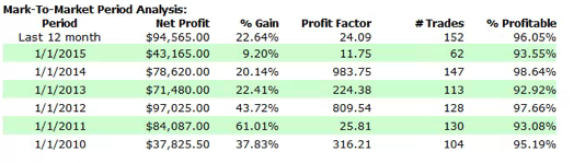
How Analysts Traditionally Value Equity

fig1I learned the traditional method for producing equity valuations in the 1980’s, from  Chase bank’s excellent credit training program.  The standard technique was to develop several years of projected financial statements, and then discount the cash flows and terminal value to arrive at an NPV. I’m guessing the basic approach hasn’t changed all that much over the last 30-40 years and probably continues to serve as the fundamental building block for M&A transactions and PE deals.

Damadoran

Amongst several excellent texts on the topic I can recommend, for example, Aswath Damodaran’s book on valuation.

Arguably the weakest point in the methodology are the assumptions made about the long term growth rate of the business and the rate used to discount the cash flows to produce the PV.  Since we are dealing with long term projections, small variations in these rates can make a considerable difference to the outcome.

The Monte Carlo Approach

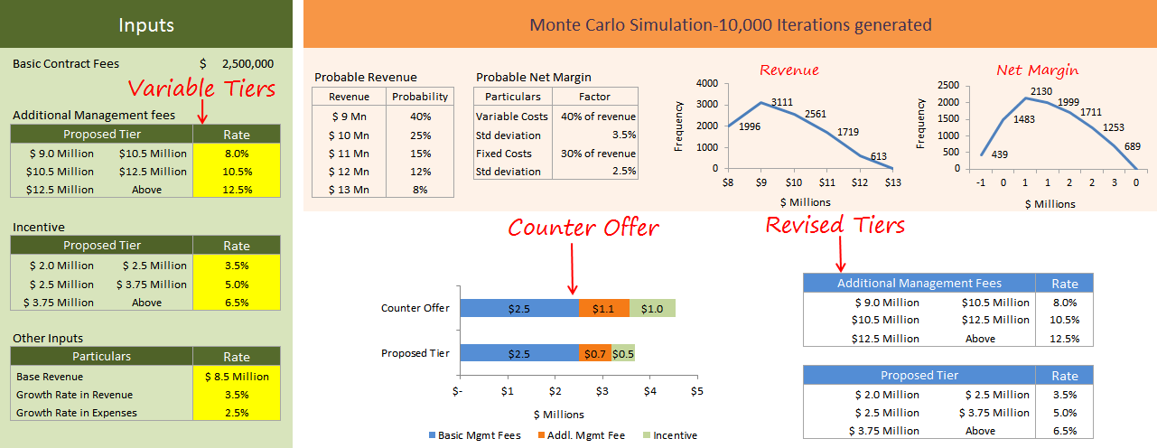
Around 20 years ago I wrote a paper titled “A New Approach to Equity Valuation”, in which I attempted to define a new methodology for equity valuation.  The idea was simple enough:  instead of guessing an appropriate rate to discount the projected cash flows generated by the company, you embed the riskiness into the cash flows themselves, using probability distributions.  That allows you to model the cash flows using Monte Carlo simulation and discount them using the risk-free rate, which is much easier to determine.  In a similar vein,  the model can allow for stochastic growth rates, perhaps also taking into account the arrival of potential new entrants, or disruptive technologies.

I recall taking the idea to an acquaintance of mine who at the time was head of M&A at a prestigious boutique bank in London.  About five minutes into the conversation I realized I had lost him at “Monte Carlo”.  It was yet another instance of the gulf between the fundamental and quantitative approach to investment finance, something I have always regarded as rather artificial.  The line has blurred in several places over the last few decades – option theory of the firm and factor models, to name but two examples – but remains largely intact.  I have met very few equity analysts who have the slightest clue about quantitative research and vice-versa, for that matter.  This is a pity in my view, as there is much to be gained by blending knowledge of the two disciplines.

SSALGOTRADING AD

The basic idea of the Monte Carlo approach is to formulate probability distributions for key variables that drive the business, such as sales, gross margin, cost of goods, etc., as well as related growth rates. You then determine the outcome in terms of P&L and cash flows over a large number of simulations, from which you can derive a probability distribution for the firm/equity value.

npv

There are two potential sources of data one can use to build a Monte Carlo model: the historical distributions of the variables and information from line management. It is the latter that is likely to be especially useful, because you can embed management’s expertise and understanding of the business and its competitive environment directly into the model variables, rather than relying upon a single discount rate to account for all the possible sources of variation in the cash flows.

It can get a little complicated, of course: one cannot simply assume that all the variables evolve independently – COGS is likely to fall as a % of sales as sales increase, for example, due to economies of scale. Such interactive effects are critically important and it is necessary to dig deep into the inner workings of the business to model them successfully.  But to those who may view such a task as overwhelmingly complicated I can offer several counter examples.  For instance, in the 1970’s  I worked on large scale simulation models of the North Sea oil fields that incorporated volumes of information from geology to engineering to financial markets.  Another large scale simulation was built to assess how best to manage tanker traffic at one of the world’s busiest sea ports.

Creating a simulation model of  the financials of a single firm is a simple task, by comparison. And, after you have built the model it will typically remain fundamentally unchanged in basic form for many years making the task of producing valuation estimates much easier in future.

Applications of Monte Carlo Methods in Equity Valuation

Ok, so what’s the point?  At the end of the day, don’t you just end up with the same result as from traditional methods, i.e. an estimate of the equity or firm value? Actually no – what you have instead is an estimate of the probability distribution of the value, something decidedly more useful.

For example:

Contract Negotiation

Monte Carlo methods have been applied successfully to model contract negotiation scenarios, for instance for management consulting projects, where several rounds of negotiation are often involved in reaching an agreed pricing structure.

Negotiation

 Stock Selection

You might build a portfolio of value stocks whose share price is below the median value, in the expectation that the majority of the universe will prove to be undervalued, over the long term.  Or you might embed information about the expected value of the equities in your universe (and their cashflow volatilities) into you portfolio construction model.

Private Equity / Mergers & Acquisitions

In a PE or M&A negotiation your model provides a range of values to select from, each of which is associated with an estimated “probability of overpayment”.  For example, your opening bid might be a little below the median value, where it is likely that you are under-bidding for the projected cash flows.  That allows some headroom to increase the bid, if necessary, without incurring too great a risk of over-paying.

Recent Research

A survey of recent research in the field yields some interesting results, amongst them a paper by Magnus Pedersen entitled Monte Carlo Simulation in Financial Valuation (2014).  Pedersen takes a rather different approach to applying Monte Carlo methods to equity valuation.   Specifically, he uses the historical distribution of the price/book ratio to derive the empirical distribution of the equity value rather than modeling the individual cash flows.  This is a sensible compromise for someone who, unlike an analyst at a major sell-side firm, may not have access to management information necessary to build a more sophisticated model.  Nevertheless, Pedersen is able to demonstrate quite interesting results using MC methods to construct equity portfolios (weighted according to the Kelly criterion), in an accompanying paper Portfolio Optimization & Monte Carlo Simulation (2014).

For those who find the subject interesting, Pedersen offers several free books on his web site, which are worth reviewing.

cover_strategies-sp500

Designing a Scalable Futures Strategy

I have been working on a higher frequency version of the eMini S&P 500 futures strategy, based on 3-minute bar intervals, which is designed to trade a couple of times a week, with hold periods of 2-3 days.  Even higher frequency strategies are possible, of course, but my estimation is that a hold period of under a week provides the best combination of liquidity and capacity.  Furthermore, the strategy is of low enough frequency that it is not at all latency sensitive – indeed, in the performance analysis below I have assumed that the market must trade through the limit price before the system enters a trade (relaxing the assumption and allowing the system to trade when the market touches the limit price improves the performance).

The other important design criteria are the high % of profitable trades and Kelly f (both over 95%).  This enables the investor to employ money management techniques, such a fixed-fractional allocation for example, in order to scale the trade size up from 1 to 10 contracts, without too great a risk of a major drawdown in realized P&L.

The end result is a strategy that produces profits of $80,000 to $100,000 a year on a 10 contract position, with an annual rate of return of 30% and a Sharpe ratio in excess of 2.0.

Furthermore, of the 682 trades since Jan 2010, only 29 have been losers.

Annual P&L (out of sample)

Annual PL


Equity Curve

EC

Strategy Performance

Perf 1

What’s the Downside?

Everything comes at a price, of course.  Firstly, the strategy is long-only and, by definition, will perform poorly in falling markets, such as we saw in 2008.  That’s a defensible investment thesis, of course – how many $billions are invested in buy and hold strategies? – and, besides, as one commentator remarked, the trick is to develop multiple strategies for different market regimes (although, sensible as that sounds, one is left with the difficulty of correctly identifying the market regime).

The second drawback is revealed by the trade chart below, which plots the drawdown experienced during each trade.  The great majority of these drawdowns are unrealized, and in most cases the trade recovers to make a profit.  However, there are some very severe cases, such as Sept 2014, when the strategy experienced a drawdown of $85,000 before recovering to make a profit on the trade.  For most investors, the agony of risking an entire year’s P&L just to make a few hundred dollars would be too great.

SSALGOTRADING AD

It should be pointed out that the by the time the drawdown event took place the strategy had already produced many hundreds of thousands of dollars of profit.  So, one could take the view that by that stage the strategy was playing with “house money” and could well afford to take such a risk.

One obvious “solution” to the drawdown problem is to use some kind of stop loss. Unfortunately, the effect is simply to convert an unrealized drawdown into a realized loss.  For some, however, it might be preferable to take a hit of $40,000 or $50,000 once every few years, rather than suffer the  uncertainty of an even larger potential loss.  Either way, despite its many pleasant characteristics, this is not a strategy for investors with weak stomachs!

Trade

Money Management – the Good, the Bad and the Ugly

The infatuation of futures traders with the subject of money management, (more aptly described as position sizing), is something of a puzzle for someone coming from a background in equities or forex.  The idea is, simply, that one can improve one’s  trading performance through the judicious use of leverage, increasing the size of a position at times and reducing it at others.

MM Grapgic

Perhaps the most widely known money management technique is the Martingale, where the size of the trade is doubled after every loss.  It is easy to show mathematically that such a system must win eventually, provided that the bet size is unlimited.  It is also easy to show that, small as it may be, there is a non-zero probability of a long string of losing trades that would bankrupt the trader before he was able to recoup all his losses.  Still, the prospect offered by the Martingale strategy is an alluring one: the idea that, no matter what the underlying trading strategy, one can eventually be certain of winning.  And so a virtual cottage industry of money management techniques has evolved.

One of the reasons why the money management concept is prevalent in the futures industry compared to, say, equities or f/x, is simply the trading mechanics.  Doubling the size of a position in futures might mean trading an extra contract, or perhaps a ten-lot; doing the same in equities might mean scaling into and out of multiple positions comprising many thousands of shares.  The execution risk and cost of trying to implement a money management program in equities has historically made the  idea infeasible, although that is less true today, given the decline in commission rates and the arrival of smart execution algorithms.  Still, money management is a concept that originated in the futures industry and will forever be associated with it.

SSALGOTRADING AD

Van Tharp on Position Sizing
I was recently recommended to read Van Tharp’s Definitive Guide to Position Sizing, which devotes several hundred pages to the subject.  Leaving aside the great number of pages of simulation results, there is much to commend it.  Van Tharp does a pretty good job of demolishing highly speculative and very dangerous “money management” techniques such as the Kelly Criterion and Ralph Vince’s Optimal f, which make unrealistic assumptions of one kind or another, such as, for example, that there are only two outcomes, rather than the multiple possibilities from a trading strategy, or considering only the outcome of a single trade, rather than a succession of trades (whose outcome may not be independent).  Just as  with the Martingale, these techniques will often produce unacceptably large drawdowns.  In fact, as I have pointed out elsewhere, the use of leverage which many so-called money management techniques actually calls for increases in the risk in the original strategy, often reducing its risk-adjusted return.

As Van Tharp points out, mathematical literacy is not one of the strongest suits of futures traders in general and the money management strategy industry reflects that.

But Van Tharp  himself is not immune to misunderstanding mathematical concepts.  His central idea is that trading systems should be rated according to its System Quality Number, which he defines as:

SQN  = (Expectancy / standard deviation of R) * square root of Number of Trades

R is a central concept of Van Tharp’s methodology, which he defines as how much you will lose per unit of your investment.  So, for example, if you buy a stock today for $50 and plan to sell it if it reaches $40,  your R is $10.  In cases like this you have a clear definition of your R.  But what if you don’t?  Van Tharp sensibly recommends you use your average loss as an estimate of R.

Expectancy, as Van Tharp defines it, is just the expected profit per trade of the system expressed as a multiple of R.  So

SQN = ( (Average Profit per Trade / R) / standard deviation (Average Profit per Trade / R) * square root of Number of Trades

Squaring both sides of the equation, we get:

SQN^2  =  ( (Average Profit per Trade )^2 / R^2) / Variance (Average Profit per Trade / R) ) * Number of Trades

The R-squared terms cancel out, leaving the following:

SQN^2     =  ((Average Profit per Trade ) ^ 2 / Variance (Average Profit per Trade)) *  Number of Trades

Hence,

SQN = (Average Profit per Trade / Standard Deviation (Average Profit per Trade)) * square root of Number of Trades

There is another name by which this measure is more widely known in the investment community:  the Sharpe Ratio.

On the “Optimal” Position Sizing Strategy
In my view,  Van Tharp’s singular achievement has been to spawn a cottage industry out of restating a fact already widely known amongst investment professionals, i.e. that one should seek out strategies that maximize the Sharpe Ratio.

Not that seeking to maximize the Sharpe Ratio is a bad idea – far from it.  But then Van Tharp goes on to suggest that one should consider only strategies with a SQN of greater than 2, ideally much higher (he mentions SQNs of the order of 3-6).

But 95% or more of investable strategies have a Sharpe Ratio less than 2.  In fact, in the world of investment management a Sharpe Ratio of 1.5 is considered very good.  Barely a handful of funds have demonstrated an ability to maintain a Sharpe Ratio of greater than 2 over a sustained period (Jim Simon’s Renaissance Technologies being one of them).  Only in the world of high frequency trading do strategies typically attain the kind of Sharpe Ratio (or SQN) that Van Tharp advocates.  So while Van Tharp’s intentions are well meaning, his prescription is unrealistic, for the majority of investors.

One recommendation of Van Tharp’s that should be taken seriously is that there is no single “best” money management strategy that suits every investor.  Instead, position sizing should be evolved through simulation, taking into account each trader or investor’s preferences in terms of risk and return.  This makes complete sense: a trader looking to make 100% a year and willing to risk 50% of his capital is going to adopt a very different approach to money management, compared to an investor who will be satisfied with a 10% return, provided his risk of losing money is very low.  Again, however, there is nothing new here:  the problem of optimal allocation based on an investor’s aversion to risk has been thoroughly addressed in the literature for at least the last 50 years.

What about the Equity Curve Money Management strategy I discussed in a previous post?  Isn’t that a kind of Martingale?  Yes and no.  Indeed, the strategy does require us to increase the original investment after a period of loss. But it does so, not after a single losing trade, but after a series of losses from which the strategy is showing evidence of recovering.  Furthermore, the ECMM system caps the add-on investment at some specified level, rather than continuing to double the trade size after every loss, as in a Martingale.

But the critical difference between the ECMM and the standard Martingale lies in the assumptions about dependency in the returns of the underlying strategy. In the traditional Martingale, profits and losses are independent from one trade to the next.  By contrast, scenarios where ECMM is likely to prove effective are ones where there is dependency in the underlying strategy, more specifically, negative autocorrelation in returns over some horizon.  What that means is that periods of losses or lower returns tend to be followed by periods of gains, or higher returns.  In other words, ECMM works when the underlying strategy has a tendency towards mean reversion.

CONCLUSION
The futures industry has spawned a myriad of position sizing strategies.  Many are impractical, or positively dangerous, leading as they do to significant risk of catastrophic loss.  Generally, investors should seek out strategies with higher Sharpe Ratios, and use money management techniques only to improve the risk-adjusted return.  But there is no universal money management methodology that will suit every investor.  Instead, money management should be conditioned on each individual investors risk preferences.